Download
1 / 1
10 likes | 165 Views
Precision = N est #points on the estimated contour N act #points on the actual contour Latency = argmax i (P i ) P i Path length of i th tracing sensor Indicator of energy consumed.

E N D
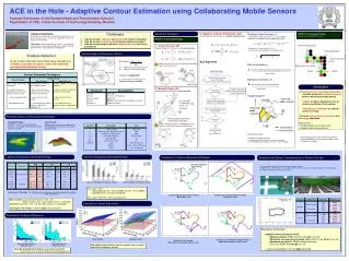
Precision = Nest #points on the estimated contour Nact #points on the actual contour Latency=argmaxi(Pi) Pi Path length of ith tracing sensor Indicator of energy consumed ACE in the Hole - Adaptive Contour Estimation using Collaborating Mobile Sensors Sumana Srinivasan, Krithi Ramamritham and Purushottam Kulkarni Department of CSE, Indian Institute of Technology Bombay, Mumbai. Movement Strategies • 3. Adaptive Contour Estimation ACE • Choose direction that minimizes the adaptive spread function • ACE Algorithm Contour Estimation Estimation of the boundary formed by connecting a set of points of equal value in a field e.g., temperature, pressure, pollutant concentration Applications: Estimating extent of oil spills - a prerequisite for containment and corrective action (as in figure), tracking pollutant flows, study of plankton assemblages Challenges How do sensors approach and surround the contour efficiently? How do sensors co-ordinate for distributed contour estimation? How do sensors adapt to different deployments, sizes and shapes of contours? STEP 2: Coverage Phase Use wall moving algorithm to trace • Distance from Contour, • Use Nonlinear regression to fit (xi, yi,zi) and compute coefficients using Nelder Mead simplex optimization • Estimate (xˆ, yˆ) such that f((xˆ, yˆ) = • If (x,y) is the current position of the sensor, then • Size of contour, . • = Area of envelope bounding estimated points on contour • Area of field • Spread of sensors, S • S = Area of convex hull of current positions • Area of field • Target Angle ' • Estimating centroid • Centroid of envelope bounding • estimated points on contour if sensors converge or • estimated convergence points if sensors not converged. STEP 1: Converge Phase • 1. Direct Descent DD • Choose direction that minimizes the distance function • Latency high when sensors are collocated and contour • is big. Need to spread!! System Model and Evaluation Metrics Problem Definition Given a scalar field with varying field value, the task is to estimate a contour of a given value with maximum precision and minimum latency Contour Estimation Techniques Remote Sensing In-situ Sensing Static Sensors Mobile Sensors Uses image processing for estimation. • Low accuracy due to obstructions and inclement weather affect accuracy • Large coverage possible • High deployment cost Combine local samples to form a global estimate. • High density and large number of sensors for high accuracy and coverage • Low sensor cost and energy • Cannot adapt to dynamic contours, high cost of redeployment Exploit mobility to increase samples. • Fewer sensors can yield high accuracy and coverage • Higher sensor cost and energy • Can adapt to dynamic contours without redeployment Conclusions • ACE provides best-of-both-worlds solution • Enables sensors to intelligently choose between direct descent and spread • Adapts to type of deployment, size of contour and distance from contour • Distributed co-ordination for efficient contour coverage • Performs high precision, low latency and low energy estimation • Other Issues • Handle limited transmission range • Support discontinuous contours • 2. Spread Always SA • Choose direction that minimizes spread function • Latency high when sensors are deployed far and • contour is small. Need to spread judiciously!! Parameter Assumptions Contour Sensor Communication Energy Movement Continuous Error free,, self-localized Single-hop Mobility+Communication+Computation+ Sensing Step-wise discrete Evaluation Setup and Simulation Parameters Pollutant Field WQMAP - a tool for simulating pollutant dispersion, Three pollutant load sites, 120 time steps for simulation Light Field Measurements taken at every grid point on 15x15 grid with three light sources using Crossbow Mote Parameter Description Value l nmax nsim nest rsense Rtrans Contours Length of grid Maximum steps allowed per sensor Number of simulation runs Estimation frequency Sensing radius Transmission range Large Medium Small 500, 140 2000 1000 Every 5 steps √2 √l > 50% of field area > 10% - 50% of field area < 10% of field area Acknowledgement: We thank Parmesh Ramanathan, Sachitanand Malewar, Amey Apte and GRAM++ team at IITB for their support. Precision Comparison (Bounded Energy) Latency Comparison (Unbounded Energy) Comparison of Sensors Movement Strategies Feasibility and Energy Characterization on Robotic Test bed Contours Deployment ACE DD SA • 11x8 grid with granularity 8 cm with single slit neon source. • ATMEGA 128, 11MHz processor, 2.4GHz CDMA, 3 white line sensors, 2 shaft encoders, 2 ultra low power DC motors, rotating arm with 2 servo motors Latency CP Latency CP Latency CP Large Medium Small Non-clustered 139 2 498 11 248 8 100 100 100 142 2 681 15 268 7 100 71 63 229 4 780 16 319 7 100 78 29 Large Medium Small Clustered 375 8 845 23 276 25 100 99 96 441 5 1006 17 319 7 100 31 11 483 5 1119 12 326 11 78 22 4 Non-clustered deployment (Medium contour) Clustered deployment (Medium contour) • Max. steps > 100: • Non-clustered: ACE > DD by 20-25% and ACE > SA by 25-30% • Clustered: ACE > DD and SA by 30-45% • Max. steps ≤ 100: ACE DD for all deployments Convergence Percentage, CP = Number of runs at least one sensor converged on the contour Total number of runs Sensors directly approach the contour DD Latency = 818 Sensors only spread around the centroid SA Latency = 623 Contours Deployment Algorithm Total Energy Non-clustered: Large and Small contours: ACE DD Medium contour: ACE < DD by 22% and ACE < SA by 38% Clustered: All contours, ACE < DD by 7-12% and ACE < SA by 4-20% Convergence Percentage is uniformly higher than DD and SA Medium Non-clustered Clustered ACE DD ACE DD 2030J Sensitivity to Design Parameters 2700J 3342J 3890J Small Non-clustered Clustered ACE DD ACE DD 1249J Distribution of Latency Differences 1335J 1417J 1587J • Summary of Results • Adaptive Contour Estimation (ACE) • Minimizeslatency7-22% over DD and 4-38% over SA • Maximizesconvergence percentage 8-45% over DD and 30-62% over SA • Maximizesprecision by 15-40% for bounded steps • Consumes 7-24%less energy over DD • Latency and prediction error are highly correlated Medium Contour Small Contour Sensors 1,5,7,9 redirected without overlap ACE (with redirection) Latency = 383 Sensors 7 and 8 overlap ACE (without redirection) Latency = 451 Non-clustered deployment (Medium contour) Clustered deployment (Medium contour) ACE adapts best to distance from the contour, size of contour and extent of spread of sensors Very high probability that ACE has lesser latency than DD - Factor of 6 for non-clustered and 8 for clustered deployments