Download
1 / 78
780 likes | 928 Views
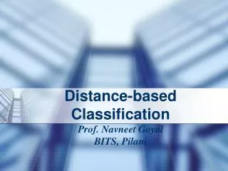
Clustering Prof. Navneet Goyal BITS, Pilani. Inter-cluster distances are maximized. Intra-cluster distances are minimized. What is Cluster Analysis?.

E N D
Inter-cluster distances are maximized Intra-cluster distances are minimized What is Cluster Analysis? • Finding groups of objects such that the objects in a group will be similar (or related) to one another and different from (or unrelated to) the objects in other groups Source of figure: unknown
Clustering • Clustering of data is a method by which large sets of data is grouped into clusters of smaller sets of similar data • Objects in one cluster have high similarity to each other and are dissimilar to objects in other clusters • An example of unsupervised learning • Group objects that share common characteristics
Clustering Applications • Segmentcustomer database based on similar buying patterns. • Group houses in a town into neighborhoods based on similar features. • Identify new plant species • Identify similar Web usage patterns
Clustering Applications • Marketing: Help marketers discover distinct groups in their customer bases, and then use this knowledge to develop targeted marketing programs • Land use: Identification of areas of similar land use in an earth observation database • Insurance: Identifying groups of motor insurance policy holders with a high average claim cost • City-planning: Identifying groups of houses according to their house type, value, and geographical location • Earth-quake studies: Observed earth quake epicenters should be clustered along continent faults
Applications of Cluster Analysis • Understanding • Group related documents for browsing, group genes and proteins that have similar functionality, or group stocks with similar price fluctuations • Summarization • Reduce the size of large data sets Clustering precipitation in Australia
Applications of Cluster Analysis • Many years ago, during a cholera outbreak in London, a physician plotted the location of cases on amap, getting a plot that looked like Fig. 14. Properly visualized, the data indicated that cases clustered around certain intersections, where there were polluted wells, not only exposing the cause of cholera, but indicating what to do about the problem. Alas, not all data mining is this easy, often because the clusters are in so many dimensions that visualization is very hard.
Applications of Cluster Analysis • Skycat clustered 2x10⁹ sky objects into stars, galaxies, quasars, etc. Each object was a point in aspace of 7 dimensions, with each dimension representing radiation in one band of the spectrum. The Sloan Sky Survey is a more ambitious attempt to catalog and cluster the entire visible universe. • Documents may be thought of as points in a high-dimensional space, where each dimension corresponds to one possible word. The position of a document in a dimension is the number of times the word occurs in the document (or just 1 if it occurs, 0 if not). Clusters of documents in this space often correspond to groups of documents on the same topic.
Clustering Example Source: Data Mining by Dunham, M H
Size Based Geographic Distance Based Clustering Houses Source of figure: Data Mining by Dunham, M H
How many clusters? Six Clusters Two Clusters Four Clusters Notion of a Cluster can be Ambiguous Source of figure: Introduction to Data Mining by Tan et. al.
Clustering vs. Classification • No prior knowledge • Number of clusters • Meaning/interpretation of clusters • Unsupervised learning
Types of Data in Cluster Analysis Data matrix
Types of Data in Cluster Analysis Dissimilarity Matrix
Dissimilarity Matrix • Many clustering algorithms operate on dissimilarity matrix • If data matrix is given, it needs to be transformed into a dissimilarity matrix first • How can we assess dissimilarity d(i,j)?
Types of Data • Interval-scaled variables • Binary variables • Nominal, ordinal, and ratio variables • Variables of mixed types
Interval-scaled Variables • Continuous measurements of a roughly linear scale • Weight, height, latitude and longitude coordinates, temperature, etc. • Effect of measurement units in attributes • Smaller unit Larger variable range Larger effect to the clustering structure • Standardization + background knowledge • Clustering BB player may require giving more weightage to height
Standardizing Variables • Standardize data • Calculate the mean absolute deviation: where • Calculate the standardized measurement (z-score) • Using mean absolute deviation is more robust than using standard deviation as z-scores of outliers do not become too small and so they remain detectable
Binary Variables • A contingency table for binary data • Simple matching coefficient (invariant, if the binary variable is symmetric): • Jaccard coefficient (noninvariant if the binary variable is asymmetric): Object j Object i
Dissimilarity between Binary Variables • Example • gender is a symmetric attribute • the remaining attributes are asymmetric binary • let the values Y and P be set to 1, and the value N be set to 0
Nominal Variables • A generalization of the binary variable in that it can take more than 2 states, e.g., red, yellow, blue, green • Method 1: Simple matching • m: # of matches, p: total # of variables • Method 2: use a large number of binary variables • creating a new binary variable for each of the M nominal states
Ordinal Variables • An ordinal variable can be discrete or continuous • order is important, e.g., rank • Can be treated like interval-scaled • replacing xif by their rank • map the range of each variable onto [0, 1] by replacing i-th object in the f-th variable by • compute the dissimilarity using methods for interval-scaled variables
Ratio-Scaled Variables • Ratio-scaled variable: a positive measurement on a nonlinear scale, approximately at exponential scale, such as AeBt or Ae-Bt • Methods: • treat them like interval-scaled variables — not a good choice! (why?) • apply logarithmic transformation yif = log(xif) • treat them as continuous ordinal data treat their rank as interval-scaled.
Variables of Mixed Types • A database may contain all the six types of variables • symmetric binary, asymmetric binary, nominal, ordinal, interval and ratio. • One may use a weighted formula to combine their effects. • f is binary or nominal: dij(f) = 0 if xif = xjf , or dij(f) = 1 o.w. • f is interval-based: use the normalized distance • f is ordinal or ratio-scaled • compute ranks rif and • and treat zif as interval-scaled
Similarity Measures If i = (xi1, xi2, …, xip,) and j = (xj1, xj2, …, xjp) are two p-dimensional data objects, then • Euclidean distance • Manhattan distance • Minkowski distance
What Is Good Clustering? • A good clustering method will produce high quality clusters with • high intra-class similarity • low inter-class similarity • The quality of a clustering result depends on both the similarity measure used by the method and its implementation. • The quality of a clustering method is also measured by its ability to discover some or all of the hidden patterns.
Impact of Outliers on Clustering Source of figure: Data Mining by Dunham, M H
Problems with Outliers • Many clustering algorithms take as input the number of clusters • Some clustering algorithms find and eliminate outliers • Statistical techniques to detect outliers • Discordancy Test • Not very realistic for real life data
Clustering Problem • Given a database D={t1,t2,…,tn} of tuples and an integer value k, the Clustering Problem is to define a mapping f:Dg{1,..,k} where each ti is assigned to one cluster Kj, 1<=j<=k. • A Cluster, Kj, contains precisely those tuples mapped to it. • Unlike classification problem, clusters are not known a priori.
Clustering Hierarchical Partitional Density-based Grid-based Clustering Approaches
Clustering Algorithms • K-means and its variants • Hierarchical clustering • Density-based clustering
Types of Clusterings • Important distinction between hierarchical and partitionalsets of clusters • Partitional Clustering • A division of data objects into non-overlapping subsets (clusters) such that each data object is in exactly one subset • Hierarchical clustering • A set of nested clusters organized as a hierarchical tree
A Partitional Clustering Iterative K-means, K-medoids Partitional Clustering Original Points
Hierarchical Clustering Traditional Hierarchical Clustering Traditional Dendrogram Non-traditional Hierarchical Clustering Non-traditional Dendrogram
Hierarchical Methods Creates a hierarchical decomposition of a given set of data objects • Agglomerative • Initially each item in its own cluster • Clusters are merged iteratively • Bottom up • Divisive • Initially all items in one cluster • Large clusters are divided successively • Top down
Step 0 Step 1 Step 2 Step 3 Step 4 agglomerative (AGNES) a a b b a b c d e c c d e d d e e divisive (DIANA) Step 3 Step 2 Step 1 Step 0 Step 4 Hierarchical Clustering
Hierarchical Clustering • Produces a set of nested clusters organized as a hierarchical tree • Can be visualized as a “dendrogram” • A tree like diagram that records the sequences of merges or splits
Density-based Methods • Most partitioning-based methods cluster objects based on distances between them • Can find only spherical-shaped clusters • Density-based clustering • Continue growing a given cluster as long as the density in the ‘neighborhood’ exceeds some threshold.
Hierarchical Algorithms • Single Link (MIN) • MST Single Link • Complete Link (MAX) • Average Link (Group Average)
Partitioning Algorithms: Basic Concept • Partitioning method: Construct a partition of a database D of n objects into a set of k clusters • Given a k, find a partition of k clusters that optimizes the chosen partitioning criterion • Global optimal: exhaustively enumerate all partitions • Heuristic methods: k-means and k-medoids algorithms • k-means (MacQueen’67): Each cluster is represented by the center of the cluster • k-medoids or PAM (Partition around medoids) (Kaufman & Rousseeuw’87): Each cluster is represented by one of the objects in the cluster
K-means • Works when we know k, the number of clusters we want to find • Idea: • Randomly pick k points as the “centroids” of the k clusters • Loop: • For each point, put the point in the cluster to whose centroid it is closest • Recompute the cluster centroids • Repeat loop (until there is no change in clusters between two consecutive iterations.) Iterative improvement of the objective function: Sum of the squared distance from each point to the centroid of its cluster
K-means Example • For simplicity, 1-dimension objects and k=2. • Numerical difference is used as the distance • Objects: 1, 2, 5, 6,7 • K-means: • Randomly select 5 and 6 as centroids; • => Two clusters {1,2,5} and {6,7}; meanC1=8/3, meanC2=6.5 • => {1,2}, {5,6,7}; meanC1=1.5, meanC2=6 • => no change. • Aggregate dissimilarity • (sum of squares of distance of each point of each cluster from its cluster center--(intra-cluster distance) • = 0.52+ 0.52+ 12+ 02+12 = 2.5 |1-1.5|2
K-Means Example • Given: {2,4,10,12,3,20,30,11,25}, k=2 • Randomly choose seeds: m1=3,m2=4 • K1={2,3}, K2={4,10,12,20,30,11,25}, m1=2.5,m2=16 • K1={2,3,4},K2={10,12,20,30,11,25}, m1=3,m2=18 • K1={2,3,4,10},K2={12,20,30,11,25}, m1=4.75,m2=19.6 • K1={2,3,4,10,11,12},K2={20,30,25}, m1=7,m2=25 • Stop as the clusters with these means are the same
Pick seeds Reassign clusters Compute centroids Reasssign clusters x x x Compute centroids x x x K Means Example(K=2) Reassign clusters Converged! [From Mooney]
Pros & Cons of K-means • Relatively efficient: O(tkn) n: # objects, k: # clusters, t: # iterations; k, t << n. • Applicable only when mean is defined • What about categorical data? • Need to specify the number of clusters • Unable to handle noisy data and outliers
Problems with K-means • Need to know k in advance • Could try out several k? • Unfortunately, cluster tightness increases with increasing K. The best intra-cluster tightness occurs when k=n (every point in its own cluster) • Tends to go to local minima that are sensitive to the starting centroids • Try out multiple starting points • Disjoint and exhaustive • Doesn’t have a notion of “outliers” • Outlier problem can be handled by K-medoid or neighborhood-based algorithms • Assumes clusters are spherical in vector space • Sensitive to coordinate changes, weighting etc. Example showing sensitivity to seeds In the above, if you start with B and E as centroids you converge to {A,B,C} and {D,E,F} If you start with D and F you converge to {A,B,D,E} {C,F}
Good Initial Centroids Source of figure: Introduction to Data Mining by Tan et. al.
Poor Initial Centroids Source of figure: Introduction to Data Mining by Tan et. al.