Download
1 / 30
310 likes | 522 Views
1. The importance of the firm’s production function, the relationship between quantity of inputs and quantity of output 2. Why production is often subject to diminishing returns to inputs

E N D
1. The importance of the firm’s production function, the relationship between quantity of inputs and quantity of output 2. Why production is often subject to diminishing returns to inputs 3. The various types of costs a firm faces and how they generate the firm’s marginal and average cost curves 4. Why a firm’s costs may differ in the short run versus the long run 5. How the firm’s technology of production can generate increasing returns to scale Chapter 11 Behind the Supply Curve: Inputs and Costs
The Production Function • A production function is the relationship between the quantity of inputs a firm uses and the quantity of output it produces. • A fixed input is an input whose quantity is fixed for a particular period and cannot be varied. • A variable input is an input whose quantity the firm can vary at any time. Inputs and Output • The long run is the period in which all inputs can be varied. • The short run is the period in which at least one input is fixed. • The total product curve shows how the quantity of output depends on the quantity of the variable input, for a given quantity of the fixed input.
Production Function and TP Curve for George and Martha’s Farm Quantity of wheat (bushels) Adding a 7th worker leads to an increase in output of only 7 bushels MP of labor Quantity of labor L Quantity of wheat Q D L MPL D Q / = (worker) (bushels) (bushels per worker) Total Product, TP Adding a 2nd worker leads to an increase in output of 17 bushels 0 0 100 19 1 19 17 2 36 80 15 3 51 13 60 4 64 11 5 75 9 40 6 84 7 7 91 20 5 8 96 0 1 2 3 4 5 6 7 8 Quantity of labor (workers) Although the total product curve in the figure slopes upward along its entire length, the slope isn’t constant: as you move up the curve to the right, it flattens out due to changing marginal product of labor.
Marginal Product of Labor • The marginal product of an input is the additional quantity of output that is produced by using one more unit of that input.
GLOBAL COMPARISON: Wheat Yields Around The World • The disparity between France and the United States is striking, given that they are both wealthy countries with comparable agricultural technology. • In the United States, farmers receive payments from the government to supplement their incomes, but European farmers benefit from price floors. • In poor countries like Uganda and Ethiopia, foreign aid can lead to significantly depressed yields. • Foreign aid from wealthy countries has often taken the form of surplus food, which depresses local market prices, severely hurting the local agriculture that poor countries normally depend on.
Marginal Product of Labor Curve There are diminishing returns to an input when an increase in the quantity of that input, holding the levels of all other inputs fixed, leads to a decline in the marginal product of that input. The following marginal product of labor curve illustrates this concept clearly. Marginal product of labor (bushels per worker) 19 17 15 13 11 There are diminishing returns to labor. 9 7 5 Marginal product of labor, MPL 0 1 2 3 4 5 6 7 8 Quantity of labor (workers) Here, the first worker employed generates an increase in output of 19 bushels, the second worker generates an increase of 17 bushels, and so on…
Total Product, Marginal Product, and the Fixed Input Marginal product of labor (bushels per worker) Quantity of wheat (bushels) 160 30 TP 140 20 25 120 20 TP 100 10 15 80 60 10 40 MPL 20 5 20 MPL 10 0 1 2 3 4 5 6 7 8 0 1 2 3 4 5 6 7 8 Quantity of labor (workers) Quantity of labor (workers) (a) Total Product Curves (b) Marginal Product Curves With more land, each worker can produce more wheat. So an increase in the fixed input shifts the total product curve up from TP10 to TP20. This shift also implies that the marginal product of each worker is higher when the farm is larger. As a result, an increase in acreage also shifts the marginal product of labor curve up from MPL10 to MPL20.
Pitfalls What’s a Unit? • The marginal product of labor (or any other input) is defined as the increase in the quantity of output when you increase the quantity of that input by one unit. • What do we mean by a “unit” of labor? Is it an additional hour of labor, an additional week, or a person-year? • The answer is that it doesn’t matter, as long as you are consistent. • One common source of error in economics is getting units confused—say, comparing the output added by an additional hour of labor with the cost of employing a worker for a week. • Whatever units you use, always be careful that you use the same units throughout your analysis of any problem.
From the Production Function to Cost Curves • A fixed cost is a cost that does not depend on the quantity of output produced. It is the cost of the fixed input. • A variable cost is a cost that depends on the quantity of output produced. It is the cost of the variable input. Total Cost Curve • The total cost of producing a given quantity of output is the sum of the fixed cost and the variable cost of producing that quantity of output. TC = FC + VC • The total cost curve becomes steeper as more output is produced due to diminishing returns.
Total Cost Curve for George and Martha’s Farm Cost Total cost, TC $2,000 I 1,800 H 1,600 G 1,400 F 1,200 E 1,000 D 800 C 600 B 400 A 200 0 19 36 51 64 75 84 91 96 Quantity of wheat (bushels) Variable cost (VC) Total cost Quantity of labor L Quantity of wheat Q Point on graph Fixed Cost (FC) (worker) (TC = FC + VC) (bushels) A 0 0 $ O $400 $ 400 B 1 19 200 400 600 C 2 36 400 400 800 D 3 51 600 400 1,000 E 4 64 800 400 1,200 F 5 75 1,000 400 1,400 G 6 84 1,200 400 1,600 H 7 91 1,400 400 1,800 I 8 96 1,600 400 2,000
Two Key Concepts: Marginal Cost and Average Cost • As in the case of marginal product, marginal cost is equal to rise(the increase in total cost) divided by run(the increase in the quantity of output).
Total Cost and Marginal Cost Curves for Selena’s Gourmet Salsas (a) Total Cost (b) Marginal Cost Cost of case Cost 8th case of salsa increases total cost by $180. $1,400 T C $250 MC 1,200 2nd case of salsa increases total cost by $36. 200 1,000 150 800 600 100 400 50 200 0 1 2 3 4 5 6 7 8 9 10 0 1 2 3 4 5 6 7 8 9 10 Quantity of salsa (cases) Quantity of salsa (cases)
Why is the Marginal Cost Curve Upward Sloping? • The marginal cost curve is upward sloping because there are diminishing returns to inputs in this example. As output increases, the marginal product of the variable input declines. • This implies that more and more of the variable input must be used to produce each additional unit of output as the amount of output already produced rises. • And since each unit of the variable input must be paid for, the cost per additional unit of output also rises. Average Cost • Average total cost, often referred to simply as average cost, is total cost divided by quantity of output produced. ATC = TC/Q = (Total Cost) / (Quantity of Output) • A U-shaped average total cost curve falls at low levels of output, then rises at higher levels. • Average fixed cost is the fixed cost per unit of output. AFC = FC/Q = (Fixed Cost) / (Quantity of Output) • Average variable cost is the variable cost per unit of output. AVC = VC/Q= (Variable Cost) / (Quantity of Output)
Average Cost Average Total Cost (ATC) • Increasing output, therefore, has two opposing effects on average total cost—the spreading effect and the diminishing returns effect: • The spreading effect: the larger the output, the greater the quantity of output over which fixed cost is spread, leading to lower the average fixed cost • The diminishing returns effect: the larger the output, the greater the amount of variable input required to produce additional units leading to higher average variable cost Average Cost • Average fixed cost is the fixed cost per unit of output. AFC = FC/Q = (Fixed Cost) / (Quantity of Output) • Average variable cost is the variable cost per unit of output. AVC = VC/Q= (Variable Cost) / (Quantity of Output)
Average Total Cost Curve for Selena’s Gourmet Salsas Cost of case $140 Average total cost, ATC Minimum average total cost 120 100 M 80 60 40 20 0 1 2 3 4 5 6 7 8 9 10 Quantity of salsa (cases) Minimum-cost output
Putting the Four Cost Curves Together Note that: Marginal cost is upward sloping due to diminishing returns. Average variable cost also is upward sloping, but is flatter than the marginal cost curve. Average fixed cost is downward sloping because of the spreading effect. The marginal cost curve intersects the average total cost curve from below, crossing it at its lowest point. This last feature is our next subject of study.
Marginal Cost & Average Cost Curves for Selena’s Gourmet Salsas The bottom of the U curve is at the level of output at which the marginal cost curve crosses the average total cost curve from below. Is this an accident? No! Cost of case $250 MC 200 150 A T C A VC 100 M 50 AFC 0 1 2 3 4 5 6 7 8 9 10 Quantity of salsa (cases) Minimum-cost output
General Principles that Are Always True About a Firm’s Marginal and Average Total Cost Curves • The minimum-cost output is the quantity of output at which average total cost is lowest—the bottom of the U-shaped average total cost curve. • At the minimum-cost output, average total cost is equal tomarginal cost. • At output less than the minimum-cost output, marginal cost isless thanaverage total cost and average total cost is falling. • And at output greater than the minimum-cost output, marginal cost isgreater thanaverage total cost and average total cost is rising.
The Relationship Between the Average Total Cost and the Marginal Cost Curves Cost of unit MC If marginal cost is above average total cost, average total cost is rising. A T C MC H B 2 A 1 M B A 1 2 MC If marginal cost is below average total cost, average total cost is falling. L Quantity When marginal cost equals average total cost, we must be at the bottom of the U, because only at that point is average total cost neither falling nor rising.
Does the Marginal Cost Curve Always Slope Upward? • In practice, marginal cost curves often slope downward as a firm increases its production from zero up to some low level, sloping upward only at higher levels of production. • This initial downward slope occurs because a firm that employs only a few workers often cannot reap the benefits of specialization of labor. • This specialization can lead to increasing returns at first, and so to a downward-sloping marginal cost curve. • Once there are enough workers to permit specialization, however, diminishing returns set in.
More Realistic Cost Curves Cost of unit MC 2. … but diminishing returns set in once the benefits from specialization are exhausted and marginal cost rises. A T C A VC 1. Increasing specialization leads to lower marginal cost… Quantity
ECONOMICS IN ACTION Don’t Put Out the Welcome Mat • With our abundant supply of undeveloped land, real estate developers have long found it profitable to buy big parcels of land, build a large number of homes, and create entire new communities. • But what is profitable for developers is not necessarily good for the existing residents. • In the past few years, real estate developers have encountered increasingly stiff resistance from local residents because of the additional costs—the marginal costs—imposed on existing homeowners from new developments. • The local tax rate that new homeowners pay on their new homes is the same as what existing homeowners pay on their older homes. • That tax rate reflects the current total cost of services, and the taxes that an average homeowner pays reflect the average total cost of providing services to a household.
ECONOMICS IN ACTION Don’t Put Out the Welcome Mat • The average total cost of providing services is based on the town’s use of existing facilities, such as the existing school buildings, the existing number of teachers, the existing fleet of school buses, and so on. • But when a large development of homes is constructed, those facilities are no longer adequate: new schools must be built, new teachers hired, and so on. • The quantity of output increases. • So the marginal cost of providing municipal services per household associated with a new, large-scale development turns out to be much higher than the average total cost per household of existing homes. • As a result, new developments and facilities cause everyone’s local tax rate to go up.
Short-Run versus Long-Run Costs • In the short run, fixed cost is completely outside the control of a firm. But all inputs are variable in the long run: This means that in the long run fixed cost may also be varied. • In the long run, in other words, a firm’s fixed cost becomes a variable it can choose. • The firm will choose its fixed cost in the long run based on the level of output it expects to produce.
Low fixed cost (FC = $108) High fixed cost (FC = $216) Average total cost of case Average total cost of case Low variable cost High variable cost Quantity of salsa Total cost Total cost (salsa) A T C A T C 1 2 1 $ 12 $ 120 $120.00 $ 6 $222 $222.00 2 48 156 78.00 24 240 120.00 3 108 216 72.00 54 270 90.00 4 192 300 75.00 96 312 78.00 5 300 408 81.60 150 366 73.20 6 432 540 90.00 216 432 72.00 7 588 696 99.43 294 510 72.86 8 768 876 109.50 384 600 75.00 9 972 1,080 120.00 486 702 78.00 10 1,200 1,308 130.80 600 816 81.60 Choosing the Level of Fixed Cost of Selena’s Gourmet Salsas At low output levels, low fixed cost yields lower average total cost Cost of case There is a trade-off between higher fixed cost and lower variable cost for any given output level, and vice versa. But as output goes up, average total cost is lower with the higher amount of fixed cost. At high output levels, high fixed cost yields lower average total cost $250 200 Low fixed cost 150 A T C 1 100 C A T 2 High fixed cost 50 0 1 2 3 4 5 6 7 8 9 10 Quantity of salsa (cases)
Short-Run and Long-Run Average Total Cost Curves The long-run average total cost curve shows the relationship between output and average total cost when fixed cost has been chosen to minimize average total cost for each level of output. Cost of case Constant returns to scale Increasing returns to scale Decreasing returns to scale A T C A T C A T C L R A T C 3 6 9 B Y A X C 0 3 4 5 6 7 8 9 Quantity of salsa (cases)
Returns to Scale • There are increasing returns to scale (economies of scale) when long-run average total cost declines as output increases. • There are decreasing returns to scale (diseconomies of scale) when long-run average total cost increases as output increases. • There are constant returns to scale when long-run average total cost is constant as output increases.