Download
1 / 60
610 likes | 621 Views
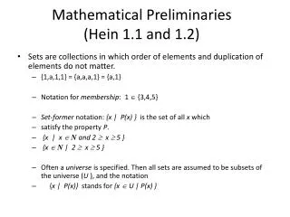
Mathematical Preliminaries. Mathematical Preliminaries Sets Functions Relations Graphs Proof Techniques. SETS. A set is a collection of elements. We write. Set Representations C = { a, b, c, d, e, f, g, h, i, j, k } C = { a, b, …, k } S = { 2, 4, 6, … }

E N D
Mathematical Preliminaries Costas Busch - RPI
Mathematical Preliminaries • Sets • Functions • Relations • Graphs • Proof Techniques Costas Busch - RPI
SETS A set is a collection of elements We write Costas Busch - RPI
Set Representations • C = { a, b, c, d, e, f, g, h, i, j, k } • C = { a, b, …, k } • S = { 2, 4, 6, … } • S = { j : j > 0, and j = 2k for some k>0 } • S = { j : j is nonnegative and even } finite set infinite set Costas Busch - RPI
U A 6 8 2 3 1 7 4 5 9 10 A = { 1, 2, 3, 4, 5 } • Universal Set: all possible elements • U = { 1 , … , 10 } Costas Busch - RPI
B A • Set Operations • A = { 1, 2, 3 } B = { 2, 3, 4, 5} • Union • A U B = { 1, 2, 3, 4, 5 } • Intersection • A B = { 2, 3 } • Difference • A - B = { 1 } • B - A = { 4, 5 } 2 4 1 3 5 U 2 3 1 Venn diagrams Costas Busch - RPI
Complement • Universal set = {1, …, 7} • A = { 1, 2, 3 } A = { 4, 5, 6, 7} 4 A A 6 3 1 2 5 7 A = A Costas Busch - RPI
{ even integers } = { odd integers } Integers 1 odd 0 5 even 6 2 4 3 7 Costas Busch - RPI
DeMorgan’s Laws A U B = A B U A B = A U B U Costas Busch - RPI
Empty, Null Set: = { } S U = S S = S - = S - S = U = Universal Set Costas Busch - RPI
U A B U A B Subset A = { 1, 2, 3} B = { 1, 2, 3, 4, 5 } Proper Subset: B A Costas Busch - RPI
A B = U Disjoint Sets A = { 1, 2, 3 } B = { 5, 6} A B Costas Busch - RPI
Set Cardinality • For finite sets A = { 2, 5, 7 } |A| = 3 (set size) Costas Busch - RPI
Powersets A powerset is a set of sets S = { a, b, c } Powerset of S = the set of all the subsets of S 2S = { , {a}, {b}, {c}, {a, b}, {a, c}, {b, c}, {a, b, c} } Observation: | 2S | = 2|S| ( 8 = 23 ) Costas Busch - RPI
Sequences and Tuples • A sequence of objects is a list of these objects in some order. • We usually designate a sequence by writing the list within parentheses. • For example, the sequence 7, 21, 57 would be written: (7, 21, 57). • The order doesn’t matter in a set, but in a sequence it does. Hence (7, 21, 57) is not the same as (57, 7, 21). Costas Busch - RPI
Sequences and Tuples • Repetition does matter in a sequence, but it doesn’t matter in a set. • (7, 7, 21, 57) is different from both of the other sequences, whereas the set {7, 21, 57} is identical to the set {7, 7, 21, 57}. • As with sets, sequences may be finite or infinite. Costas Busch - RPI
Sequences and Tuples • Finite sequences often are called tuples. • A sequence with k elements is a k-tuple. • Thus (7, 21, 57) is a 3-tuple. • A 2-tuple is also called an ordered pair. Costas Busch - RPI
Cartesian Product A = { 2, 4 } B = { 2, 3, 5 } A X B = { (2, 2), (2, 3), (2, 5), ( 4, 2), (4, 3), (4, 5) } |A X B| = |A| |B| Generalizes to more than two sets A X B X … X Z Costas Busch - RPI
Exercise • If A is the set {0, 1}, • What is the power set of A. • What is The set of all ordered pairs of A. • If A = {1, 2} and B = {x, y, z}, • find AxB • Find AxBxA Costas Busch - RPI
FUNCTIONS domain range B 4 A f(1) = a a 1 2 b c 3 5 f : A -> B If A = domain then f is a total function otherwise f is a partial function Costas Busch - RPI
RELATIONS R = {(x1, y1), (x2, y2), (x3, y3), …} xi R yi e. g. if R = ‘>’: 2 > 1, 3 > 2, 3 > 1 Costas Busch - RPI
Equivalence Relations • Reflexive: x R x • Symmetric: x R y y R x • Transitive: x R y and y R z x R z • Example: R = ‘=‘ • x = x • x = y y = x • x = y and y = z x = z Costas Busch - RPI
Equivalence Classes For equivalence relation R equivalence class of x = {y : x R y} Example: R = { (1, 1), (2, 2), (1, 2), (2, 1), (3, 3), (4, 4), (3, 4), (4, 3) } Equivalence class of 1 = {1, 2} Equivalence class of 3 = {3, 4} Costas Busch - RPI
GRAPHS A directed graph e b node d a edge c • Nodes (Vertices) • V = { a, b, c, d, e } • Edges • E = { (a,b), (b,c), (b,e),(c,a), (c,e), (d,c), (e,b), (e,d) } Costas Busch - RPI
Labeled Graph 2 6 e 2 b 1 3 d a 6 5 c Costas Busch - RPI
e b d a c Walk Walk is a sequence of adjacent edges (e, d), (d, c), (c, a) Costas Busch - RPI
e b d a c Path Path is a walk where no edge is repeated Simple path: no node is repeated Costas Busch - RPI
Cycle e base b 3 1 d a 2 c Cycle: a walk from a node (base) to itself Simple cycle: only the base node is repeated Costas Busch - RPI
Euler Tour 8 base e 7 1 b 4 6 5 d a 2 3 c A cycle that contains each edge once Costas Busch - RPI
Hamiltonian Cycle 5 base e 1 b 4 d a 2 3 c A simple cycle that contains all nodes Costas Busch - RPI
Finding All Simple Paths e b d a c origin Costas Busch - RPI
Step 1 e b d a c origin (c, a) (c, e) Costas Busch - RPI
Step 2 e b d a (c, a) (c, a), (a, b) (c, e) (c, e), (e, b) (c, e), (e, d) c origin Costas Busch - RPI
Step 3 e b d a c (c, a) (c, a), (a, b) (c, a), (a, b), (b, e) (c, e) (c, e), (e, b) (c, e), (e, d) origin Costas Busch - RPI
Step 4 e b d a (c, a) (c, a), (a, b) (c, a), (a, b), (b, e) (c, a), (a, b), (b, e), (e,d) (c, e) (c, e), (e, b) (c, e), (e, d) c origin Costas Busch - RPI
Trees root parent leaf child Trees have no cycles Costas Busch - RPI
root Level 0 Level 1 Height 3 leaf Level 2 Level 3 Costas Busch - RPI
Binary Trees Costas Busch - RPI
Strings and Languages • Strings of characters are fundamental building blocks in computer science. • The alphabet over which the strings are defined may vary with the application. • For our purposes, we define an alphabet to be any nonempty finite set. • The members of the alphabet are the symbols of the alphabet. Costas Busch - RPI
Strings and Languages • We generally use capital Greek letters Σ and Γ to designate alphabets and a typewriter font for symbols from an alphabet. • The following are a few examples of alphabets. • Σ1 = {0,1} • Σ2 = {a, b, c, d, e, f, g, h, i, j, k, l, m, n, o, p, q, r, s, t, u, v, w, x, y, z} • Γ = {0, 1, x, y, z} Costas Busch - RPI
Strings and Languages • A string over an alphabet is a finite sequence of symbols from that alphabet, usually written next to one another and not separated by commas. • If Σ1 = {0,1}, then 01001 is a string over Σ1. • If Σ2 = {a, b, c,..., z}, then abracadabra is a string over Σ2. • If w is a string over Σ, the length of w, written |w|, is the number of symbols that it contains. Costas Busch - RPI
Strings and Languages • The string of length zero is called the empty string and is written ε. • The empty string plays the role of 0 in a number system. • If w has length n, we can write w = w1w2 ··· wn where each wi ∈ Σ. • The reverse of w, written wR, is the string obtained by writing w in the opposite order (i.e., wnwn−1 ··· w1). • String z is a substring of w if z appears consecutively within w. For example, cad is a substring of abracadabra. Costas Busch - RPI
Strings and Languages • If we have string x of length m and string y of length n, the concatenation of x and y, written xy, is the string obtained by appending y to the end of x, as in x1 ··· xmy1 ··· yn. • To concatenate a string with itself many times, we use the superscript notation xk to mean k . Costas Busch - RPI
Strings and Languages • The lexicographic order of strings is the same as the familiar dictionary order. • We’ll occasionally use a modified lexicographic order, called shortlex order or simply string order, that is identical to lexicographic order, except that shorter strings precede longer strings. • Thus the string ordering of all strings over the alphabet {0,1} is (ε, 0, 1, 00, 01, 10, 11, 000,...). Costas Busch - RPI
Boolean Logic • Boolean logic is a mathematical system built around the two values TRUE and FALSE. • Though originally conceived of as pure mathematics, this system is now considered to be the foundation of digital electronics and computer design. • The values TRUE and FALSE are called the Boolean values and are often represented by the values 1 and 0. • We use Boolean values in situations with two possibilities, such as a wire that may have a high or a low voltage, a proposition that may be true or false, or a question that may be answered yes or no. Costas Busch - RPI
Boolean Logic • We can manipulate Boolean values with the Boolean operations. • The simplest Boolean operation is the negation or NOT operation, designated with the symbol ¬. • The negation of a Boolean value is the opposite value. • Thus ¬0=1 and ¬1=0. Costas Busch - RPI
Boolean Logic • We designate the conjunction or AND operation with the symbol ∧. The conjunction of two Boolean values is 1 if both of those values are 1. • The disjunction or OR operation is designated with the symbol ∨. The disjunction of two Boolean values is 1 if either of those values is 1. Costas Busch - RPI
Boolean Logic • The exclusive or, or XOR, operation is designated by the ⊕ symbol and is 1 if either but not both of its two operands is 1. • The equality operation, written with the symbol ↔, is 1 if both of its operands have the same value. • Finally, the implication operation is designated by the symbol → and is 0 if its first operand is 1 and its second operand is 0; otherwise, → is 1. • We summarize this information as follows: Costas Busch - RPI
Boolean Logic Costas Busch - RPI
PROOF TECHNIQUES • Proof by induction • Proof by contradiction Costas Busch - RPI