Download
1 / 20
200 likes | 285 Views
This article presents a method for solving language equations efficiently using partitioned representations. Includes problem formulation, example of traffic light controller, and solution process based on partitioned representation with experimental results and conclusions.

E N D
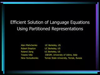
Efficient Solution of Language Equations Using Partitioned Representations Alan Mishchenko UC Berkeley, US Robert Brayton UC Berkeley, US Roland Jiang UC Berkeley, US Tiziano Villa DIEGM, University of Udine, Italy Nina YevtushenkoTomsk State University,Tomsk, Russia
Overview • Problem formulation • Example: Traffic light controller • Partitioned representation • Solution based on partitioned representation • Experimental results • Conclusion
i1 FSM FSM o1 FSM FSM o2 i2 FSM FSM FSM Spec Fixed o i u v Unknown Problem Formulation Specification S (i,o) Fixed F (i,v,u,o) Unknown X (u,v) Problem: Given S and F, find the Most General Solution (MGS) X of Solution:
Combinational Network is a DAG Node has single output Node is a logic function Sequential Network is arbitrary Node has many outputs Node is an FSM i1 FSM FSM o1 i1 FSM logic FSM logic o2 i2 o1 FSM FSM logic FSM logic o2 i2 logic logic logic Combinational and Sequential Flexibility X Y
Computing Most General FSM Solution Input: Prefix-closed specification S(i,o) and fixed part F(i,v,u,o) Output: Most general FSM (prefix-closed progressive) solution X begin 01 X := Complete( S ) 02 X := Determinize( X ) 03 X := Complement( X ) 04 X := Support( X, (i,v,u,o) ) 05 X := Product( Complete(F), X ) 06 X := Support( X, (u,v) ) 07 X := Determinize( X ) 08 X := Complete( X ) 09 X := Complement( X ) 10 X := PrefixClose( X ) 11 X := Progressive( X, u ) 12 return X end
Example: Traffic Light Controller Synthesis General Topology This example Specification Specification S S I O z Fixed Traffic Light F F V U v Unknown Controller X X
Traffic Light Controller (Fixed Part) .model fixed .inputs v z .outputs Acc .mv v 2 wait go .mv z 3 red green yellow .mv CS, NS 3 Fr Fg Fy .latch NS CS .reset CS Fr .table ->Acc 1 .table v z CS ->NS wait red Fr Fr go red Fr Fg wait green Fg Fg go green Fg Fy wait yellow Fy Fy go yellow Fy Fr .end z = {red, green, yellow} v = {wait, go} Specification S z Traffic Light F v Controller X
Traffic Light Controller (Specification) .model spec .inputs z .outputs Acc .mv z 3 red green yellow .mv CS,NS 4 S1 S2 S3 S4 .table ->Acc 1 .latch NS CS .reset CS S1 .table z CS ->NS red S1 S2 red S2 S3 green S3 S4 yellow S4 S1 .end z = {red, green, yellow} v = {wait, go} Specification S z Traffic Light F v Controller X
Traffic Light Controller (Synthesis Script) echo "Synthesis ..." determinize -lci spec.mva spec_dci.mva support v(2),z(3) spec_dci.mva spec_dci_supp.mva support v(2),z(3) fixed.mva fixed_supp.mva product -l fixed_supp.mva spec_dci_supp.mva p.mva supportv(2) p.mva p_supp.mva determinize -lci p_supp.mva p_dci.mva progressive-i 0 p_dci.mva x.mva echo "Verification ..." support v(2),z(3) x.mva x_supp.mva product x_supp.mva fixed_supp.mva prod.mva support v(2),z(3) spec.mva spec_supp.mva check prod.mva spec_supp.mva
Traffic Light Controller (Solution) .model solution .inputs v .outputs Acc .mv v 2 wait go .mv CS, NS 4 \ FrS1 FrS2 FgS3 FyS4 .latch NS CS .reset CS FrS1 .table ->Acc 1 .table v CS ->NS wait FrS1 FrS2 go FrS2 FgS3 go FgS3 FyS4 go FyS4 FrS1 .end z = {red, green, yellow} v = {wait, go} Specification S z Traffic Light F v Controller X
o u i1 Latches FSM FSM o1 ns FSM FSM o2 i2 FSM FSM FSM cs i v Spec Fixed o i u v Unknown Partitioned Representation Fixed part: Output functions:oj = Oj(i,v,cs) Transition functions:nsk = NSk(i,v,cs) Communication functions:um= Um(i,v,cs)
Computing with Partitioned Representation • Completion • Complementation • Product computation • Changing support • Determinization (subset construction)
Completion The output relation is O(i,o,cs) = j[oj Oj(i,cs)] For each current state cs, the transitions are not defined iff P(i,o) =cs[O(i,o,cs) &(cs)] Using partitioned representation, this computation becomes P(i,o) =cs[j[oj Oj(i,cs)] &(cs)] This is a partitioned image computation. Any image computation method can be used.
Complementation • For non-deterministic automata, requires determinization • For deterministic automata, make non-accepting states accepting, and vice versa • In the case of partitioned representation, the don’t-care state becomes acceptable, other states become non-acceptable
Product Computation • Combine the partitions of the two components
Changing Support (Lifting and Projecting) • Expanding support is trivial • Reducing support requires existential quantification • In general, cannot be done on the partitioned representation • Therefore, postponed until the determinization step
Determinization (Subset Construction) Start with the subset containing only the initial state. For each subset , compute the subsets reachable through (u, v). Define the acceptance relation: Compute the condition of the transition is into non-accepting states: Restrict the transitions to those that are not contained in Q(u, v): Direct the transition under Q(u, v) to DCN. Complete and redirect the remaining transitions to DCA.
Experimental Results Name is the ISCAS benchmark name i/o/cs is the number of input/output/state variables Fcs/Xcs is the partitioning of the state variables States(X) is the number of states in the solution Mono is the runtime of the monolithic computation in seconds Part is the runtime of partitioned computation is in seconds Ratio is improvement due to the proposed method
Conclusions • Introduced language solving problems • Showed a simple example • Discussed partitioned representation • Presented experimental results
Future Work • Developing methods for finding a particular solution contained in the most general solution • Developing efficient sequential synthesis methods without state space traversal