Download

1 / 17
170 likes | 208 Views
6. Taxes – Government Policy. Taxes. How taxes on sellers affect market outcomes Taxes discourage market activity Smaller quantity sold Buyers and sellers share the burden of tax Buyers pay more Worse off Sellers receive less Get the higher price but pay the tax

E N D
6 Taxes – Government Policy
Taxes • How taxes on sellers affect market outcomes • Taxes discourage market activity • Smaller quantity sold • Buyers and sellers share the burden of tax • Buyers pay more • Worse off • Sellers receive less • Get the higher price but pay the tax • Overall: effective price fall • Worse off
Taxes • How taxes on buyers affect market outcomes • Initial impact on the demand • Demand curve shifts left • Lower equilibrium price • Lower equilibrium quantity • The tax – reduces the size of the market
7 Equilibrium with tax A tax on buyers Tax ($0.50) Price of Ice-Cream Cone A tax on buyers shifts the demand curve downward by the size of the tax ($0.50). Equilibrium without tax Price buyers pay Price without tax $3.30 2.80 3.00 Price sellers receive 100 90 D2 Supply, S1 0 Quantity of Ice-Cream Cones When a tax of $0.50 is levied on buyers, the demand curve shifts down by $0.50 from D1 to D2. The equilibrium quantity falls from 100 to 90 cones. The price that sellers receive falls from $3.00 to $2.80. The price that buyers pay (including the tax) rises from $3.00 to $3.30. Even though the tax is levied on buyers, buyers and sellers share the burden of the tax. D1
Taxes • How taxes on buyers affect market outcomes • Buyers and sellers share the burden of the tax • Sellers get a lower price • Worse off • Buyers pay a lower market price • Effective price (with tax) rises • Worse off • Taxes levied on sellers and taxes levied on buyers are equivalent
Can congress distribute the burden of a payroll tax? • Payroll taxes • Deducted from the amount you earned • By law, the tax burden: • Half of the tax - paid by firms • Out of firm’s revenue • Half of the tax - paid by workers • Deducted from workers’ paychecks • Tax incidence analysis • Payroll tax = tax on a good • Good = labor • Price = wage
Can congress distribute the burden of a payroll tax? • Introduce payroll tax • Wage received by workers falls • Wage paid by firms rises • Workers and firms share the burden of the tax • Not necessarily fifty-fifty as the legislation requires • Lawmakers • Can decide whether a tax comes from the buyer’s pocket or from the seller’s • Cannot legislate the true burden of a tax • Tax incidence: forces of supply and demand
8 A payroll tax Wage Tax wedge Wage firms pay Wage without tax Wage workers receive Labor supply 0 Quantity of Labor A payroll tax places a wedge between the wage that workers receive and the wage that firms pay. Comparing wages with and without the tax, you can see that workers and firms share the tax burden. This division of the tax burden between workers and firms does not depend on whether the government levies the tax on workers, levies the tax on firms, or divides the tax equally between the two groups. Labor demand
Taxes • Elasticity and tax incidence • Dividing the tax burden • Very elastic supply and relatively inelastic demand • Sellers – small burden of tax • Buyers – most of the burden • Relatively inelastic supply and very elastic demand • Sellers – most of the tax burden • Buyers – small burden
9 How the burden of a tax is divided (a) Price (a) Elastic Supply, Inelastic Demand 1. When supply is more elastic than demand . . . Tax 2. . . . The incidence of the tax falls more heavily on consumers . . . 3. . . . Than on producers. Price buyers pay Price without tax Price sellers receive 0 Quantity Supply In panel (a), the supply curve is elastic, and the demand curve is inelastic. In this case, the price received by sellers falls only slightly, while the price paid by buyers rises substantially. Thus, buyers bear most of the burden of the tax. Demand
9 How the burden of a tax is divided (b) Price (b) Inelastic Supply, Elastic Demand 1. When demand is more elastic than supply . . . 3. Than on consumers Tax 2. . . . The incidence of the tax falls more heavily on producers. Price buyers pay Price without tax Price sellers receive Demand 0 Quantity Supply In panel (b), the supply curve is inelastic, and the demand curve is elastic. In this case, the price received by sellers falls substantially, while the price paid by buyers rises only slightly. Thus, sellers bear most of the burden of the tax.
Taxes • Tax burden - falls more heavily on the side of the market that is less elastic • Small elasticity of demand • Buyers do not have good alternatives to consuming this good • Small elasticity of supply • Sellers do not have good alternatives to producing this good
Who pays the luxury tax? • 1990 - new luxury tax • Goal: to raise revenue from those who could most easily afford to pay • Luxury items • Demand - quite elastic • Supply - relatively inelastic • Outcome: • Burden of a tax falls largely on the suppliers • 1993 – most of the luxury tax – repealed
Elasticity of Demandeffect of a tax • Cigarettes (US)[41] • -0.3 to -0.6 (General) • -0.6 to -0.7 (Youth) – proportion of income? • Soft drinks • -0.8 to -1.0 (general)[51] (broadly defined) • -3.8 (Coca-Cola)[52] (narrow) • -4.4 (Mountain Dew)[52] (narrow) • Car fuel[45] • -0.25 (Short run) (same car – reduce trips) • -0.64 (Long run) (new car?)
Availability and closeness of substitutes “better/closer” substitute makes it to switch Results in either Greater movement along the demand curve (own) Greater shift of the demand curve (cross) Time More time to adjust, more options you can find Long-run elasticity > short-run Proportion of Income spent on the good Larger proportion -> more sensitive to changes in Income What Affects Own-Price Demand Elasticity?
3 Major Types for Demand Own-price Measures the change in quantity demanded with a change in the (own) good’s price Always negative (F.L.O.D) Always expressed in absolute value (as it’s always negative) Cross-price Measures the change in quantity demanded with a change in the price of a related good (e.g. complement or substitute) Complement (-) Substitute (+) Income Measures the change in quantity demanded with a change in income Normal/superiors goods (+) Inferior goods (-) Elasticity Measures
Own-price Larger absolute value (|e| > 1) Large changes in Qd with small changes in price Close substitutes exist (pepsi/coke) Or much consumption is discretionary (micro-brews) Cross-price Large value (e >1) Close (or good) substitute for good exists Complements Large absolute value (|e| > 1) Consumption in fixed proportions Income >1 superior (luxury?) good >0 normal < 0 inferior (Animal beer) What Does the Magnitude of the Elasticity Tell Us?