Free-Trade Equilibrium

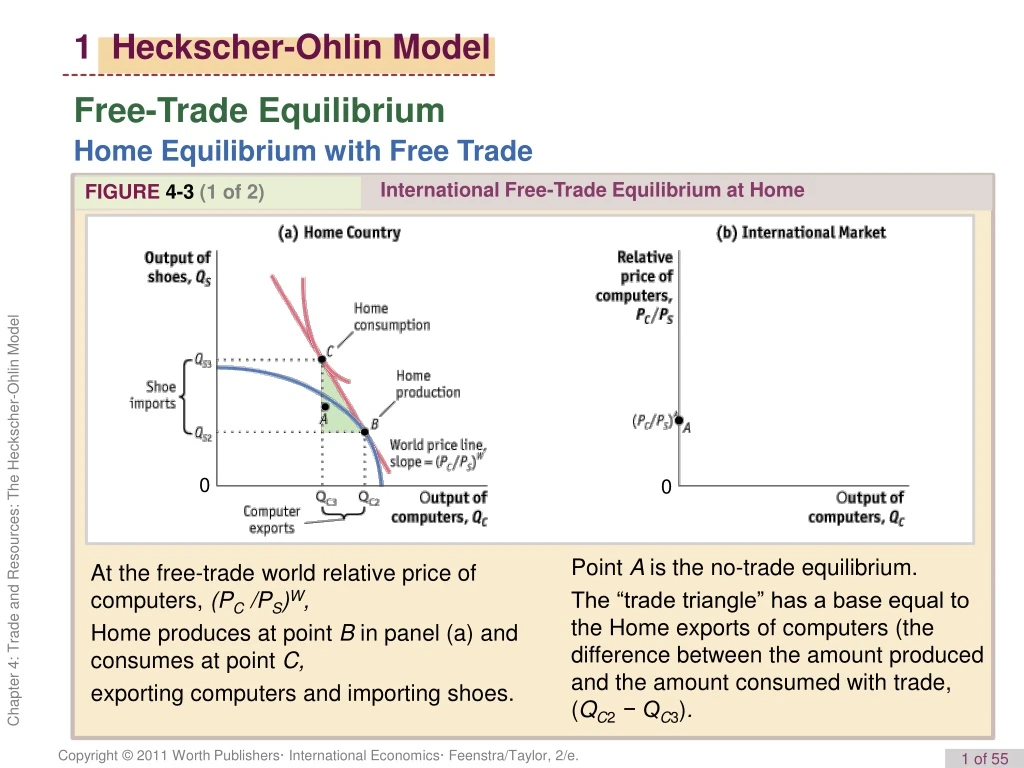
1. 1 Heckscher-Ohlin Model Free-Trade Equilibrium Home Equilibrium with Free Trade International Free-Trade Equilibrium at Home FIGURE 4-3 (1 of 2) 0 0 Point A is the no-trade equilibrium. The “trade triangle” has a base equal to the Home exports of computers (the difference between the amount produced and the amount consumed with trade, (QC2 − QC3). At thefree-trade world relative price of computers, (PC /PS)W, Homeproduces at point B in panel (a) and consumes at point C, exporting computers and importing shoes.

2. 1 Heckscher-Ohlin Model Free-Trade Equilibrium Home Equilibrium with Free Trade International Free-Trade Equilibrium at Home (continued) FIGURE 4-3 (2 of 2) 0 0 In panel (b), we showHome exports of computers equal to zero at the no-trade relative price, (PC /PS)A, and equal to (QC2 − QC3) at the free-trade relative price, (PC/PS)W. The height of this triangle is the Home imports of shoes (the difference between the amount consumed of shoes and the amount produced with trade, QS3 − QS2).

3. 1 Heckscher-Ohlin Model Free-Trade Equilibrium Foreign Equilibrium with Free Trade International Free-Trade Equilibrium in Foreign FIGURE 4-4 (1 of 2) 0 0 Point A* is the no-trade equilibrium.) The “trade triangle” has a base equal to Foreign imports of computers (the difference between the consumption of computers and the amount produced with trade, (Q*C3 − Q*C2). At the free-trade world relative price of computers, (PC /PS)W, Foreign produces at point B* in panel (a) and consumes at point C*, importing computers and exporting shoes.

4. 1 Heckscher-Ohlin Model Free-Trade Equilibrium Foreign Equilibrium with Free Trade International Free-Trade Equilibrium in Foreign (continued) FIGURE 4-4 (2 of 2) 0 0 In panel (b), we show Foreign imports of computers equal to zero at the no-trade relative price, (P*C /P*S)A*, and equal to (Q*C3 − Q*C2) at the free-trade relative price, (PC /PS)W. The height of this triangle is Foreign exports of shoes (the difference between the production of shoes and the amount consumed with trade, Q*S2 – Q*S3).

5. 1 Heckscher-Ohlin Model Free-Trade Equilibrium Equilibrium Price with Free Trade Because exports equal imports, there is no reason for the relative price to change and so this is a free-trade equilibrium. Determination of the Free-Trade World Equilibrium Price FIGURE 4-5 The world relative price of computers in the free-trade equilibrium is determined at the intersection of the Home export supply and Foreign import demand, at point D. At this relative price, the quantityof computers that Home wants to export, (QC2 − QC3), just equals the quantity ofcomputers that Foreign wants to import, (Q*C3 − Q*C2). 0

6. 1 Heckscher-Ohlin Model Free-Trade Equilibrium • Pattern of Trade • Home exports computers, the good that uses intensively the factor of production (capital) found in abundance at Home. • Foreign exports shoes, the good that uses intensively the factor of production (labor) found in abundance there. • This important result is called the Heckscher-Ohlin theorem.

7. 1 Heckscher-Ohlin Model Heckscher-Ohlin Theorem: Assumption 1: Labor and capital flow freely between the industries. Assumption 2: The production of shoes is labor-intensive as compared with computer production, which is capital-intensive. Assumption 3: The amounts of labor and capital found in the two countries differ, with Foreign abundant in labor and Home abundant in capital. Assumption 4: There is free international trade in goods. Assumption 5: The technologies for producing shoes and computers are the same across countries. Assumption 6: Tastes are the same across countries.

8. 2 Testing the Heckscher-Ohlin Model The first test of the Heckscher-Ohlin theorem was performed by economist Wassily Leontief in 1953. Leontief supposed correctly that in 1947 the United States was abundant in capital relative to the rest of the world. Thus, from the Heckscher-Ohlin theorem, Leontief expected that the United States would export capital-intensive goods and import labor-intensive goods. What Leontief actually found, however, was just the opposite: the capital–labor ratio for U.S. imports was higher than the capital–labor ratio found for U.S. exports! This finding contradicted the Heckscher-Ohlin theorem and came to be called Leontief’s paradox.

9. 2 Testing the Heckscher-Ohlin Model Leontief’s Paradox Leontief’s Test TABLE 4-1 Leontief used the numbers in this table to test the Heckscher-Ohlin theorem. Each column shows the amount of capital or labor needed to produce $1 million worth of exports from, or imports into, the United States in 1947. As shown in the last row, the capital–labor ratio for exports was less than the capital–labor ratio for imports, which is a paradoxical finding.

10. 2 Testing the Heckscher-Ohlin Model Leontief’s Paradox Explanations ■ U.S. and foreign technologies are not the same, in contrast to what the HO theorem and Leontief assumed. ■ By focusing only on labor and capital, Leontief ignored land abundance in the United States. ■ Leontief should have distinguished between skilled and unskilled labor (because it would not be surprising to find that U.S. exports are intensive in skilled labor). ■ The data for 1947 may be unusual because World War II had ended just two years earlier. ■ The United States was not engaged in completely free trade, as the Heckscher-Ohlin theorem assumes.

11. 2 Testing the Heckscher-Ohlin Model Factor Endowments in the New Millennium To determine whether a country is abundant in a certain factor, we compare the country’s share of that factor with its share of world GDP. If its share of a factor exceeds its share of world GDP, then we conclude that the country is abundant in that factor, and if its share in a certain factor is less than its share of world GDP, then we conclude that the country is scarce in that factor.

12. China Drawing High-Tech Research from U.S. For years, many of China’s best and brightest left for the United States, where high-tech industry was more cutting-edge. But Mark R. Pinto is moving in the opposite direction. Mr. Pinto is the first chief technology officer of a major American tech company to move to China. Applied Materials, is one of Silicon Valley’s most prominent firms. It supplied equipment used to perfect the first computer chips. Not just drawn by China’s markets, Western companies are also attracted to China’s huge reservoirs of cheap, highly skilled engineers. HEADLINES

13. 2 Testing the Heckscher-Ohlin Model Factor Endowments in the New Millennium Capital, Labor and Land Abundance FIGURE 4-6 Country Factor Endowments, 2000 Shown here are country shares of six factors of production in the year 2000, for eight selected countries and the rest of the world. In the first bar graph, we see that 24% of the world’s physical capital in 2000 was located in the United States, with 9% located in China, 13% located in Japan, and so on. In the final bar graph, we see that in 2000 the United States had 22% of world GDP, China had 11%, Japan had 8%, and so on.

14. 2 Testing the Heckscher-Ohlin Model Differing Productivities across Countries Remember that in the original formulation of the paradox, Leontief had found that the United States was exporting labor-intensive products even though it was capital-abundant at that time. One explanation for this outcome would be that labor is highly productive in the United States and less productive in the rest of the world. If that is the case, then the effective labor force in the United States, the labor force times its productivity (which measures how much output the labor force can produce), is much larger than it appears to be when we just count people. We can further analyze the accuracy of the H-O-model by dropping the assumption of identical technology across countries. By allowing for the differences in productivities, we can calculate a country’s effective labor force, which means how much output the labor force can produce

15. 2 Testing the Heckscher-Ohlin Model Differing Productivities across Countries Measuring Factor Abundance Once Again To allow factors of production to differ in their productivities across countries, we define the effective factor endowment as the actual amount of a factor found in a country times its productivity: Effective factor endowment = Actual factor endowment • Factor productivity

16. 2 Testing the Heckscher-Ohlin Model Differing Productivities across Countries Measuring Factor Abundance Once Again To determine whether a country is abundant in a certain factor, we compare the country’s share of that effective factor with its share of world GDP. If its share of an effective factor exceeds its share of world GDP, then we conclude that the country is abundant in that effective factor; if its share of an effective factor is less than its share of world GDP, then we conclude that the country is scarce in that effective factor. • Effective R&D Scientists • Effective R&D scientists =Actual R&D scientists • R&D spending per scientist

17. 2 Testing the Heckscher-Ohlin Model Differing Productivities across Countries Measuring Factor Abundance Once Again • Effective R&D Scientists • To account for the differences in in productivities across countries due to the availability of laboratory equipment and, we measure • EffectiveR&D Scientists =Actual R&D scientists • R&D spending per scientist

18. 2 Testing the Heckscher-Ohlin Model Differing Productivities across Countries FIGURE 4-7 (1 of 2) “Effective” Factor Endowments, 2000 Shown here are country shares of R&D scientists and land in 2000, using first the information from Figure 4.6, and then making an adjustment for the productivity of each factor across countries to obtain the “effective” shares. China was abundant in R&D scientists in 2000 (since it had 14% of the world’s R&D scientists as compared with 11% of the world’s GDP) but scarce in effective R&D scientists (because it had 7% of the world’s effective R&D scientists as compared with 11% of the world’s GDP).

19. 2 Testing the Heckscher-Ohlin Model Differing Productivities across Countries FIGURE 4-7 (2 of 2) “Effective” Factor Endowments, 2000 Shown here are country shares of R&D scientists and land in 2000, using first the information from Figure 4.6, and then making an adjustment for the productivity of each factor across countries to obtain the “effective” shares. The United States was scarce in arable land when using the number of acres (since it had 13% of the world’s land as compared with 22% of the world’s GDP) but neither scarce nor abundant in effective land (since it had 21% of the world’s effective land, which nearly equaled its share of the world’s GDP).

20. 2 Testing the Heckscher-Ohlin Model Differing Productivities across Countries Effective Arable Land TABLE 4-2 U.S. Food Trade and Total Agricultural Trade, 2000–2009 This table shows that U.S. food trade has fluctuated between positive and negative net exports since 2000, which is consistent with our finding that the United States is neither abundant nor scarce in land. Total agriculture trade (including nonfood items like cotton) has positive net exports, however.

21. 2 Testing the Heckscher-Ohlin Model Leontief’s Paradox Once Again Labor Abundance FIGURE 4-8 Labor Endowment and GDP for the United States and Rest of World, 1947 Shown here are the share of labor, “effective” labor, and GDP of the US and the rest of the world in 1947. The US had only 8% of the world’s population, as compared to 37% of the world’s GDP, so it was very scarce in labor. But when we measure effective labor by the total wages paid in each country, then the United States had 43% of the world’s effective labor as compared to 37% of GDP, so it was abundant in effective labor.

22. 2 Testing the Heckscher-Ohlin Model Leontief’s Paradox Once Again Labor Productivity Labor Productivity and Wages FIGURE 4-9 Shown here are estimated labor productivities across countries, and their wages, relative to the United States in 1990. Notice that the labor and wages were highly correlated across countries: the points roughly line up along the 45-degree line.

23. 2 Testing the Heckscher-Ohlin Model Leontief’s Paradox Once Again Labor Productivity FIGURE 4-9 (revisited) Effective Labor Abundance As suggested by Figure 4-9, wages across countries are strongly correlated with the productivity of labor. We use the wages earned by labor to measure the productivity of labor in each country. Then the effective amount of labor found in each country equals the actual amount of labor times the wage.

24. 3 Effects of Trade on Factor Prices Effect of Trade on the Wage and Rental of Home Economy-Wide Relative Demand for Labor Determination of Home equilibrium relative wage (Wage/Rental) FIGURE 4-10 The economy-wide relative demand for labor, RD, is an average of the LC /KCand LS /KScurves and lies between these curves. The relative supply, L/K, is shown by a vertical linebecause the total amount of resources in Home is fixed. The equilibrium point A, at which relative demand RD intersects relative supply L/K, determines the wage relative to the rental, W/R. 0 Relativesupply Relativedemand

25. 3 Effects of Trade on Factor Prices Effect of Trade on the Wage and Rental of Home Increase in the Relative Price of Computers Increase in the Relative Price of Computers because of free-trade FIGURE 4-11 Initially, Home is at a no-trade equilibrium at point A with a relative price of computers of (PC /PS)A. An increase in the relative price of computers to the world price, as illustrated by the steeperworld price line, (PC /PS)W, shifts production from point A to B. At point B, thereis a higher output of computers and a lower output of shoes, QC2 > QC1and QS2 < QS1. 0 Because of free-trade, Home faces a higher relative price of computers, which drives it to further specialise in the production of computers, shifting resources away from the production of shoes. The increase in the production of the capital-intensive product (computers) leads to a change in the RD for labor... Se next slide!

26. 3 Effects of Trade on Factor Prices Effect of Trade on the Wage and Rental of Home Increase in the Relative Price of Computers FIGURE 4-12 (1 of 2) Effect of a Higher Relative Price of Computers on Wage/Rental An increase in the relative price of computers shifts the economy-wide relative demand for labor, RD1, toward the relativedemand for labor in the computer industry, LC /KC. The new relative demand curve, RD2, intersects the relative supply curve for labor at a lower relative wage, (W/R)2. The new equilibrium at point B. 0

27. 3 Effects of Trade on Factor Prices Effect of Trade on the Wage and Rental of Home Increase in the Relative Price of Computers Effect of a Higher Relative Price of Computers on Wage/Rental (continued) FIGURE 4-12 (2 of 2) As a result,the wage relative to the rental falls from (W/R)1to (W/R)2. The lower relative wage causes both industries to increase their labor–capital ratios, as illustrated by the increase in both LC /KCand LS /KSat the new relative wage. The new equilibrium at point B. 0 ↑ ↓↑ ↓ Relative supplyNo change Relative demandNo change in total

28. 3 Effects of Trade on Factor Prices Determination of the Real Wage and Real Rental Change in the Real Rental R = PC• MPKCand R = PS• MPKS Because the L/K ratio increases in both industries due to the higher world relative price of computers, the marginal product of capital also increases in both industries. Rearranging the previous equation, we get MPKC = R/PC ↑ and MPKS = R/PS ↑, where R/PC (R/PS) gives the quantity of computers (shoes) a capital owner at Home can purchase with the rental. More generally, an increase in the relativ price of a product (computers) will benefit the factor of production (capital) used intensively in manufacturing that product (computers are capital-intensive).

29. 3 Effects of Trade on Factor Prices Determination of the Real Wage and Real Rental Change in the Real Wage W = PC • MPLC and W = PS • MPLS The law of diminishing returns tells us that the increase in the L/K ratio (i.e., more labor per unit of capital) will lead to a decrease in marginal product of labor in both industries. Rearranging the preceding equation, we get MPLC = W/PC ↓ and MPLS = W/PS ↓,where we see that labor experiences a decrease in real wage in terms of the quantity of computers that can be purchsed with the wage (W/PC) and the quantity of shoes that can be purchase with the wage (W/PS) at Home, and labor is clearly worse off due to the increase the relative price of computers. We can summarize our results with the following theorem, first derived by W Stolper and P Samuelson.

30. 3 Effects of Trade on Factor Prices Determination of the Real Wage and Real Rental Stolper-Samuelson Theorem: In the long run, when all factors are mobile, an increase in the relative price of a good will increase the real earnings of the factor used intensively in the production of that good and decrease the real earnings of the other factor. For our example, the Stolper-Samuelson theorem predicts that when Home opens to trade and faces a higher relative price of computers, the real rental on capital in Home rises and the real wage in Home falls. In Foreign, the changes in real factor prices are just the reverse.

31. 3 Effects of Trade on Factor Prices Changes in the Real Wage and Rental: A Numerical Example Note that shoes are more labor-intensive than computers because the share of total revenue paid to labor in shoes industry [(60/100)·100] = 60% is more than that share in computers industry [(50/100)·100]= 50%.

32. 3 Effects of Trade on Factor Prices Changes in the Real Wage and Rental: A Numerical Example General Equation for the Long-Run Change in Factor Prices The long-run results of a change in factor prices can be summarized in the following equation: Real wagefalls Real rental increases The equations relating the changes in product prices to changes in factor prices are sometimes called the “magnification effect” because they show how changes in the prices of goods have magnified effects on the earnings of factors: Real rentalfalls Real wage increases Real rentalfalls Real wage increases

33. APPLICATION Opinions toward Free Trade According to the specific-factors model, in the short run we do not know whether labor will gain or lose from free trade, but we do know that the specific factor in the export sector gains, and the specific factor in the import sector loses.

34. APPLICATION Opinions toward Free Trade We would expect that workers in export industries will support free trade (since the specific factor in that industry gains), but workers in import-competing industries will be against free trade (since the specific factor in that industry loses). In the short run, then, the industry of employment of workers will affect their attitudes toward free trade. In the long-run Heckscher-Ohlin model, however, the industry of employment should not matter.

35. APPLICATION Opinions toward Free Trade According to the Stolper-Samuelson theorem, an increase in the relative price of exports will benefit the factor of production used intensively in exports and harm the other factor, regardless of the industry in which these factors of production actually work.

36. APPLICATION Opinions toward Free Trade An increase in the relative price of exports will benefit skilled labor in the long run, regardless of whether these workers are employed in export-oriented industries or import-competing industries. In the long run, then, the skill level of workers should determine their attitudes toward free trade. In a survey conducted in the United States by the National Elections Studies (NES) in 1992, workers with lower wages or fewer years of education are more likely to favor import restrictions, whereas those with higher wages and more years of education favor free trade. ■

37. K e y T e r m KEY POINTS 1. In the Heckscher-Ohlin model, we assume that the technologies are the same across countries and that countries trade because the available resources (labor, capital, and land) differ across countries.

38. K e y T e r m KEY POINTS 2. The Heckscher-Ohlin model is a long-run framework, so labor, capital, and other resources can move freely between the industries.

39. K e y T e r m KEY POINTS 3. With two goods, two factors, and two countries, the Heckscher-Ohlin model predicts that a country will export the good that uses its abundant factor intensively and import the other good.

40. K e y T e r m KEY POINTS 4. The first test of the Heckscher-Ohlin model was made by Leontief using U.S. data for 1947. He found that U.S. exports were less capital-intensive and more labor-intensive than U.S. imports. This was a paradoxical finding because the United States was abundant in capital.

41. K e y T e r m KEY POINTS 5. The assumption of identical technologies used in the Heckscher-Ohlin model does not hold in practice. Current research has extended the empirical tests of the Heckscher-Ohlin model to allow for many factors and countries, along with differing productivities of factors across countries. When we allow for different productivities of labor in 1947, we find that the United States is abundant in effective—or skilled—labor, which explains the Leontief paradox.

42. K e y T e r m KEY POINTS 6. According to the Stolper-Samuelson theorem, an increase in the relative price of a good will cause the real earnings of labor and capital to move in opposite directions: the factor used intensively in the industry whose relative price goes up will find its earnings increased, and the real earnings of the other factor will fall.

43. K e y T e r m KEY POINTS 7. Putting together the Heckscher-Ohlin theorem and the Stolper-Samuelson theorem, we conclude that a country’s abundant factor gains from the opening of trade (because the relative price of exports goes up), and its scarce factor loses from the opening of trade.

44. K e y T e r m KEY TERMS Heckscher-Ohlin model reversal of factor intensities free-trade equilibrium Heckscher-Ohlin theorem Leontief’s paradox abundant in that factor scarce in that factor effective labor force effective factor endowment abundant in that effective factor scarce in that effective factor Stolper-Samuelson theorem,

45. K e y T e r m A P P E N D I X T O C H A P T E R 4 The Sign Test in the Heckscher-Ohlin Model Measuring the Factor Content of Trade FIGURE 4A-1 Factor Content of Trade for the United States, 1947 This table extends Leontief’s test of the Heckscher-Ohlin model to measure the factor content of net exports. The first column for exports and for imports shows the amount of capital or labor needed per $1 million worth of exports from or imports into the United States, for 1947. The second column for each shows the amount of capital or labor needed for the total exports from or imports into the United States. The final column is the difference between the totals for exports and imports. By taking the difference between the factor content of exports and the factor content of imports, we obtain the factor content of net exports, shown in the final column of Table 4A-1.

46. K e y T e r m A P P E N D I X T O C H A P T E R 4 The Sign Test in the Heckscher-Ohlin Model The Sign Test We make use of the factor content of trade in developing a test for the Heckscher-Ohlin model, called the sign test. This test states that if a country is abundant in an effective factor, then that factor’s content in net exports should be positive, but if a country is scarce in an effective factor, then that factor’s content in net exports should be negative. Sign of (country’s % share of effective factor − % share of world GDP) = Sign of country’s factor content of net exports

47. K e y T e r m A P P E N D I X T O C H A P T E R 4 The Sign Test in the Heckscher-Ohlin Model The Sign Test in a Recent Year FIGURE 4A-2 The Sign Test for 33 Countries with Differing Technologies, 1990 This table shows the sign test for the Heckscher-Ohlin model for 1990, allowing for different technologies across countries. There are 33 countries included in the study and 9 factors of production. All countries have more factors passing the sign test than failing it, especially the low- and medium-income countries. These results show that the sign test holds true when we allow productivities to differ across countries. Note: The countries with low GDP per capita are Bangladesh, Pakistan, Indonesia, Sri Lanka, Thailand, Colombia, Panama, Yugoslavia, Portugal, and Uruguay. The countries with middle GDP per capita are Greece, Ireland, Spain, Israel, Hong Kong, New Zealand, and Austria. The countries with high GDP per capita are Singapore, Italy, the United Kingdom, Japan, Belgium, Trinidad, the Netherlands, Finland, Denmark, former West Germany, France, Sweden, Norway, Switzerland, Canada, and the United States.