Download

1 / 60
600 likes | 619 Views
Discover the fascinating world of data mining and learn how to extract valuable insights from large datasets using fast methods. Explore various topics such as recursive splitting, nearest neighbor, neural networks, clustering, and association analysis.

E N D
Data Mining: What is All That Data Telling Us? Dave Dickey NCSU Statistics
What I know • What “they” can do • How “they” can do it What I don’t know • What is some particular entity doing ? • How safe is your particular information ? • Is big brother watching me right now ?
* Data being created at lightning pace * Moore’s law: (doubling / 2 years – transistors on integrated circuits) Internet “hits” Scanner cards e-mails Intercepted messages Credit scores Environmental Monitoring Satellite Images Weather Data Health & Birth Records
So we have some data – now what?? • Predict defaults, dropouts, etc. • Find buying patterns • Segment your market • Detect SPAM (or others) • Diagnose handwriting • Cluster • ANALYZE IT !!!!
Data Mining - What is it? • Large datasets • Fast methods • Not significance testing • Topics • Trees (recursive splitting) • Nearest Neighbor • Neural Networks • Clustering • Association Analysis
Trees • A “divisive” method (splits) • Start with “root node” – all in one group • Get splitting rules • Response often binary • Result is a “tree” • Example: Framingham Heart Study
Recursive Splitting x xxxx xx x xxxxx xx x xxxxxx xxx x xxxxxxD x xxxxxxxxxxxxx x xxxD x xxx xx x xxD x xxxxxxxxxxxxxxxxD x xxxx x xx x xxxxxxxxD x xx x D xx x xxxxxxxD x xxxxxxxxx xx x xxxx x xxxxxxx xxx x xxxxxxxxxxxxxD x xx xx x xD x x xxxxxxxxxxxxx X xxxxxxxxxxxxxxD x xxxxxxxxxxxxxxxxxxxxxxxxxxxxxxx Dx x xxxxxxxxxxxxxxxxxxxxxxxxxxxxxxxx x xxDD x xxxxxxxxxx xx x xxxxxxxxxxxxxxxxxxxxxxxxxx Pr{default} =0.007 Pr{default} =0.012 Pr{default} =0.006 x xxxx xx x xxxxx xx x xxxxxx xxx x xD x xxxxxxxxxxxxxxxxxx x xxxxxxx xx x xxxxxxxxxxxxxxxxxxxxxxxx x xx x xxxxx xx D x xxxxxxxx x xx x xxxxxxxxxxxxxxxxx xxx x xx x xxxx x xxxxxxx xxx x xxxxxxxxxxxxxxxx xx x xxxxxxxxxxxxxxxx X xxxx D x xxxxxxxxxxxxxxxxxxxxxxxxxxxxxxxxxxxxxxxxx x xxxxxxxxxxxxxxxxxxxxxxxxxxxxxxxxxx x xxxxxxxxxxxxxxx xx x xxxxxxxxxxxxxxxxxxxxxxxxxx X1=Debt To Income Ratio Pr{default} =0.0001 x xxxx xx x xxxxx xx x xxxxxx xxx x xxxxxxxxxxxxxxxxxxxx x xxxxxxx xx x xxxxxxxxxxxxxxxxxxxxxxxx x xx x xxxxxxxx xx x xxxxxx x xx x xxxxxxxxxxxxxxxxxxxxxxx xx x xxxx x xxxxxxx xxx x xxxxxxxxxxxxxxxx xx x xxxxxxxxxxxxxxxxD X xxxxxxxxxxxxxxxxxxxxxxxxxxxxxxxxxxxxxxxxxxxxxx x xxxxxxxxxxxxxxxxxxxxxxxxxxxxxxxxxx x xxDD x xxxxxxxxxxxx xx x xxxxxxxxxxxxxxxxxxxxxxxxxx Pr{default} =0.003 X2 = Age
Some Actual Data • Framingham Heart Study • First Stage Coronary Heart Disease • P{CHD} = Function of: • Age - no drug yet! • Cholesterol • Systolic BP Import
Example of a “tree” All 1615 patients Split # 1: Age Systolic BP “terminal node”
How to make splits? • Which variable to use? • Where to split? • Cholesterol > ____ • Systolic BP > _____ • Goal: Pure “leaves” or “terminal nodes” • Ideal split: Everyone with BP>x has problems, nobody with BP<x has problems
Where to Split? • Maximize “dependence” statistically • We use “contingency tables” Heart Disease No Yes Heart Disease No Yes 100 100 Low BP High BP DEPENDENT INDEPENDENT
Measuring Dependence • Expect 100(150/200)=75 in upper left if independent (etc. e.g. 100(50/200)=25) Heart Disease No Yes Low BP High BP 100 100 150 50 200 How far from expectations is “too far” (significant dependence)
c2 Test Statistic Low BP High BP 100 100 150 50 200 42.67 - So what? 2(400/75)+2(400/25) = 42.67
Use Probability! “P-value” “Significance Level” (0.05)
Measuring “Worth” of a Split • P-value is probability of c2 as great as that observed if independence is true. • (Pr {c2>42.67} is 0.000000000064 • P-values all too small to understand. • Logworth = -log10(p-value) = 10.19 • Best Chi-square max logworth.
Logworth for Age Splits Age 47 maximizes logworth
How to make splits? • Which variable to use? • Where to split? • Cholesterol > ____ • Systolic BP > _____ • Idea – Pick BP cutoff to minimize p-value for c2 • What does “signifiance” mean now?
Multiple testing • 50 different BPs in data, 49 ways to split • Sunday football highlights always look good! • If he shoots enough baskets, even 95% free throw shooter will miss. • Tried 49 splits, each has 5% chance of declaring significance even if there’s no relationship.
Multiple testing a = Pr{ falsely reject hypothesis 2} a = Pr{ falsely reject hypothesis 1} Pr{ falsely reject one or the other} < 2a Desired: 0.05 probabilty or less Solution: use a = 0.05/2 Or – compare 2a to 0.05
Multiple testing • 50 different BPs in data, m=49 ways to split • Multiply p-value by 49 • Stop splitting if minimum p-value is large (logworth is small). • For m splits, logworth becomes -log10(m*p-value)
Other Split Evaluations • Gini Diversity Index • { E E E E G E G G L G} • Pick 2, Pr{different} = • 1-Pr{EE}-Pr{GG}-Pr{LL} • 1- [ 10 + 6 + 0]/45 =29/45=0.64 • { E E G L G E E G L L } • 1-[6+3+3]/45 = 33/45 = 0.73 • MORE DIVERSE, LESS PURE • Shannon Entropy • Larger more diverse (less pure) • -Si pi log2(pi) {0.5, 0.4, 0.1} 1.36 {0.4, 0.2, 0.3} 1.51 (more diverse)
Goals • Split if diversity in parent “node” > summed diversities in child nodes • Observations should be • Homogeneous (not diverse) within leaves • Different between leaves • Leaves should be diverse • Framingham tree used Gini for splits
Cross validation • Traditional stats – small dataset, need all observations to estimate parameters of interest. • Data mining – loads of data, can afford “holdout sample” • Variation: n-fold cross validation • Randomly divide data into n sets • Estimate on n-1, validate on 1 • Repeat n times, using each set as holdout.
Pruning • Grow bushy tree on the “fit data” • Classify holdout data • Likely farthest out branches do not improve, possibly hurt fit on holdout data • Prune non-helpful branches. • What is “helpful”? What is good discriminator criterion?
Goals • Want diversity in parent “node” > summed diversities in child nodes • Goal is to reduce diversity within leaves • Goal is to maximize differences between leaves • Use same evaluation criteria as for splits • Costs (profits) may enter the picture for splitting or evaluation.
Accounting for Costs • Pardon me (sir, ma’am) can you spare some change? • Say “sir” to male +$2.00 • Say “ma’am” to female +$5.00 • Say “sir” to female -$1.00 (balm for slapped face) • Say “ma’am” to male -$10.00 (nose splint)
Including Probabilities Leaf has Pr(M)=.7, Pr(F)=.3. You say: M F True Gender M F 0.7 (2) 0.7 (-10) 0.3 (-1) 0.3 (5) Expected profit is 2(0.7)-1(0.3) = $1.10 if I say “sir” Expected profit is -7+1.5 = -$5.50 (a loss) if I say “Ma’am” Weight leaf profits by leaf size (# obsns.) and sum Prune (and split) to maximize profits.
Additional Ideas • Forests – Draw samples with replacement (bootstrap) and grow multiple trees. • Random Forests – Randomly sample the “features” (predictors) and build multiple trees. • Classify new point in each tree then average the probabilities, or take a plurality vote from the trees
* Lift Chart - Go from leaf of most to least response. - Lift is cumulative proportion responding.
Regression Trees • Continuous response (not just class) • Predicted response constant in regions Predict 80 Predict 50 {47, 51, 57, 45} 50 = mean X2 Predict 130 Predict 20 Predict 100 X1
Predict Pi in cell i (it’s cell mean) • Yij jth response in cell i. • Split to minimize SiSj (Yij-Pi)2 • [sum of squared deviations from cell mean] Predict 80 Predict 50 {-3, 1, 7, -5} SSq=9+1+49+25 = 84 Predict 130 Predict 20 Predict 100
Predict Pi in cell i. • Yij jth response in cell i. • Split to minimize SiSj (Yij-Pi)2
Logistic Regression • Logistic – another classifier • Older – “tried & true” method • Predict probability of response from input variables (“Features”) • Need to insure 0 < probability < 1
Example: Shuttle Missions • O-rings failed in Challenger disaster • Low temperature • Prior flights “erosion” and “blowby” in O-rings • Feature: Temperature at liftoff • Target: problem (1) - erosion or blowby vs. no problem (0)
We can easily “fit” lines • Lines exceed 1 , fall below 0 • Model L as linear in temperature • L = a+b(temp) • Convert: p = eL/(1+eL) = ea+b(temp)/ (1+ea+b(temp)) Convert
Example: Ignition • Flame exposure time = X • Ignited Y=1, did not ignite Y=0 • Y=0, X= 3, 5, 9 10 , 13, 16 • Y=1, X = 11, 12 14, 15, 17, 25, 30 • Probability of our data is “Q” • Q=(1-p)(1-p)(1-p)(1-p)pp(1-p)pp(1-p)ppp • P’s all different p=f(exposure) • Find a,b to maximize Q(a,b)
Likelihood function (Q) -2.6 0.23
IGNITION DATA The LOGISTIC Procedure Analysis of Maximum Likelihood Estimates Standard Wald Parameter DF Estimate Error Chi-Square Pr > ChiSq Intercept 1 -2.5879 1.8469 1.9633 0.1612 TIME 1 0.2346 0.1502 2.4388 0.1184 Association of Predicted Probabilities and Observed Responses Percent Concordant 79.2 Somers' D 0.583 Percent Discordant 20.8 Gamma 0.583 Percent Tied 0.0 Tau-a 0.308 Pairs 48 c 0.792
4 right, 1 wrong 5 right, 4 wrong
Example: Framingham • X=age • Y=1 if heart trouble, 0 otherwise
Framingham The LOGISTIC Procedure Analysis of Maximum Likelihood Estimates Standard Wald Parameter DF Estimate Error Chi-Square Pr>ChiSq Intercept 1 -5.4639 0.5563 96.4711 <.0001 age 1 0.0630 0.0110 32.6152 <.0001
Neural Networks • Very flexible functions • “Hidden Layers” • “Multilayer Perceptron” output inputs Logistic function of Logistic functions Of data
Arrows represent linear combinations of “basis functions,” e.g. logistics b1 Example: Y = a + b1 p1 + b2 p2 + b3 p3 Y = 4 + p1+ 2 p2 - 4 p3
Should always use holdout sample • Perturb coefficients to optimize fit (fit data) • Eliminate unnecessary arrows using holdout data.
Terms • Train: estimate coefficients • Bias: intercept a in Neural Nets • Weights: coefficients b • Radial Basis Function: Normal density • Score: Predict (usually Y from new Xs) • Activation Function: transformation to target • Supervised Learning: Training data has response.