
Cell#1 Program Instructions. Don’t run.
E N D
Presentation Transcript
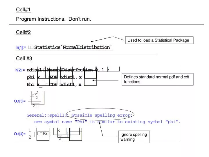
Cell#1 Program Instructions. Don’t run. Cell#2 Used to load a Statistical Package Cell #3 Defines standard normal pdf and cdf functions Ignore spelling warning
Cell #4 Clears existing values of variables that may have been used in other programs. Then defines a function that is proportional to the pdf of W and depends on ∆, f ( W, d ) where ∆ is defined by the variable d.
Cell #5 Defines actual values from relevant clinical data and parameters of interest. σ is set by s.
Cell#6 Defines the initial values for the endpoints of the integral, a & b.
Cell #7 Creates a plot of the distribution of W on [a, b]. If the plot indicates that the interval is not wide enough, values of a & b need to be manually set (trial and error) so that most of the distribution is captured before proceeding with additional Cells.
Cell#8 Defines a range of values for ∆ likely to contain the confidence interval of interest. Cell #9 Establishes the total number of points to determine the values of FQ( Wobs | X*, ∆ ) as a function of ∆. dtb is a tabulation of values for ∆ at which FQ( Wobs | X*, ∆ ) is calculated.
Cell #10 c1 is a tabulation of the reciprocal of normalization constants, which depend on the values of ∆ (symbolically represented by u). Cell #11 a1 is a tabulation by u (which symbolically represents ∆) of the area under the curve of f ( t , u ) for fixed u and over t on [– Infinity, Wobs ]. For practical purposes, the lower limit of the integral is specified as: n0(nA+nB)/((n0+nA+nB)s2)u – (b – a).
Cell #12 p1 provides a tabulation of FQ( Wobs | X*, ∆ ) by ∆. Cell #13 This cell associates each value of FQ( Wobs | X*, ∆ ) with the corresponding value of ∆. Cell #14 An interpolating function is then set to the values listed in tb.
Cell #15 A plot of the interpolating function is produced. The plot should show a reverse ‘S’ curve decreasing from near 1 to near 0. If this plot is not obtained, values of ‘upper’ and ‘lower’ (Cell 8) need to be set by the user by trial and error until the desired curve is obtained.
Cell #16 The lower bound of the confidence interval is solved by finding ∆such that FQ( Wobs | X*, ∆ ) = 1 – α / 2. In the example provided, it is – 0.7422. Cell #17 The upper bound of the confidence interval is solved by finding ∆ such that FQ( Wobs | X*, ∆ ) = α / 2. In the example provided, it is 3.6111.