Download
1 / 59
590 likes | 616 Views
Explore the principles of non-equilibrium thermodynamics and transport phenomena, including heat transfer, mass transport, and fluid mechanics. Understand the relationship between fluxes, affinities, and driving forces in non-equilibrium systems.

E N D
Using thermodynamics, we can prove that, for all positions r and r’ in a system, equilibrium is given by p(r) = p(r’) T(r) = T(r’) μ(r) = μ(r’) where p(r) is the pressure, T(r) is the temperature, and μα(r) is the chemical potential of species α atposition r. Mathematically, this tells us that the pressure, temperature, and chemical potentials areuniform in a system at equilibrium. If there is a gradient in any of these quantities, then the system is out of equilibrium. As a consequence, momentum, energy, and mass will flow through the system totry to bring it to equilibrium. Most processes that are of practicalinterest are not in equilibrium and never truly achieve equilibrium. In order to describe these systems,we need to study fluid mechanics, heat transfer, and mass transport, which are also known collectivelyas non-equilibrium thermodynamics or transport phenomena.
NON-EQLBM THERMODYNAMICS Postulate I Although system as a whole is not in eqlbm., arbitrary small elements of it are in local thermodynamic eqlbm & have state fns. which depend on state parameters through the same relationships as in the case of eqlbm states in classical eqlbm thermodynamics.
NON-EQLBM THERMODYNAMICS Postulate II Entropy gen rate fluxes affinities All sorts of transport only take place when a force, called a driving force, is applied.Transport is generally expressed as a flux J, which is defined by the amount of mass, energy,momentum, volume, or charges that are being transported pr. area pr. time.
NON-EQLBM THERMODYNAMICS Purely “resistive” systems Fluxis dependent only onaffinity at any instant at that instant System has no “memory”-
NON-EQLBM THERMODYNAMICS Coupled Phenomenon Since Jk is 0 when affinities are zero,
NON-EQLBM THERMODYNAMICS where kinetic Coeff Relationship between affinity & flux from ‘other’ sciences Postulate III
NON-EQLBM THERMODYNAMICS Postulate IV Onsager theorem {in the absence of magnetic fields}
Analysis of thermo-electric circuits Addl. Assumption : Thermo electric phenomena can be taken as LINEAR RESISTIVE SYSTEMS {higher order terms negligible} Here K = 1,2 corresp to heat flux “Q”, elec flux “e”
Analysis of thermo-electric circuits Above equations can be written as Substituting for affinities, the expressions derived earlier, we get
Defining electrical conductivity as the elec. flux per unit pot. gradient under isothermal conditions we get from above Analysis of thermo-electric circuits We need to find values of the kinetic coeffs. from exptly obtainable data.
In transport phenomena (heat transfer, mass transfer and fluid dynamics), flux is defined as the rate of flow of a property per unit area, which has the dimensions [quantity]·[time]−1·[area] j=I/A, where I=dq/dt In all cases the frequent symbol j, (or J) is used for flux, q for the physical quantity that flows, t for time, and A for area. As a mathematical concept, flux is represented by the surface integral of a vector field The surface has to be orientable, i.e. two sides can be distinguished: the surface does not fold back onto itself. Also, the surface has to be actually oriented, i.e. we use a convention as to flowing which way is counted positive; flowing backward is then counted negative. Substituting the formula of normalvector:
Fluxes • Quantity transferred through a given area per unit time • Flux occurs because of a spatial and time-varying gradient of an associatedsystemproperty. • Flux occurs in opposition to spatial gradient • Flux continues until the gradient is nullified and equilibrium is reached. • Fluxcontinuesuntilexternalforce stop • The most general relation for a flux in the x-direction is: • This relates a flux to a gradient of a property (not specically definedto be anyting at this point) • Flux is a linear response; this treatment assumes a perturbativedisplacementfromequilibrium.
Transport fluxes Eight of the most common forms of flux from the transport phenomena literature are defined as follows: Momentum flux, the rate of transfer of momentum across a unit area (N·s·m−2·s−1). (Newton's law of viscosity) Heat flux, the rate of heat flow across a unit area (J·m−2·s−1). (Fourier's law of conduction)(This definition of heat flux fits Maxwell's original definition.) Diffusion flux, the rate of movement of molecules across a unit area (mol·m−2·s−1). (Fick's law of diffusion) Volumetric flux, the rate of volume flow across a unit area (m3·m−2·s−1). (Darcy's law of groundwater flow) Mass flux, the rate of mass flow across a unit area (kg·m−2·s−1). (Either an alternate form of Fick's law that includes the molecular mass, or an alternate form of Darcy's law that includes the density.) Radiative flux, the amount of energy transferred in the form of photons at a certain distance from the source per unit area per second (J·m−2·s−1). Used in astronomy to determine the magnitude and spectral class of a star. Also acts as a generalization of heat flux, which is equal to the radiative flux when restricted to the infrared spectrum. Energy flux, the rate of transfer of energy through a unit area (J·m−2·s−1). The radiative flux and heat flux are specific cases of energy flux. Particle flux, the rate of transfer of particles through a unit area ([number of particles] m−2·s−1) These fluxes are vectors at each point in space, and have a definite magnitude and direction. Also, one can take the divergence of any of these fluxes to determine the accumulation rate of the quantity in a control volume around a given point in space. For incompressible flow, the divergence of the volume flux is zero.
NON-EQLBM THERMODYNAMICS Heat Flux : Momentum : Mass : Electricity :
Diffusion • Mass flow process by which species change their position relative to their neighbours • Driven by thermal energy and a gradient • Thermal energy → thermal vibrations → Atomic jumps Concentration / chemical potential Gradient Electric Magnetic Stress
Fick’s I law Diffusion coefficient/ diffusivity No. of atoms crossing area Aper unit time Cross-sectional area Concentration gradient Matter transport is down the concentration gradient Flow direction A • As a first approximation assume D f(t)
Steady-State Diffusion Diffusion flux does not change with time Concentration profile: Concentration (kg/m3) vs. position Concentration gradient:dC/dx (kg / m4)
Steady-State Diffusion Fick’s first law: J proportion to dC/dx D=diffusion coefficient Concentration gradient is ‘driving force’ Minus sign means diffusion is ‘downhill’: toward lower concentrations
Diffusivity (D) → f(A, B, T) Steady state diffusion D f(c) C1 Concentration → C2 D = f(c) x →
D f(c) Steady stateJ f(x,t) D = f(c) Diffusion D f(c) Non-steady stateJ = f(x,t) D = f(c)
Equations are based on the following physical principles: • Mass is conserved • Newton’s Second Law: • The First Law of thermodynamics: De = dq - dw, for a system.
Control Volume Analysis The governing equations can be obtained in the integral form by choosing a control volume (CV) in the flow field and applying the principles of the conservation of mass, momentum and energy to the CV.
Consider a differential volume element dV in the flow field. dV is small enough to be considered infinitesimal but large enough to contain a large number of molecules for continuum approach to be valid. • dV may be: • fixed in space with fluid flowing in and out of its surface or, • moving so as to contain the same fluid particles all the time. In this case the boundaries may distort and the volume may change.
Substantial derivative (time rate of change following a moving fluid element)
Control element Mass balance: u r Conservation of mass DX or
X in X Compartmental Analysis X out X is some variable of interest A change in X = X in – X out in derivative terms:
What is Diffusion? • Definition – the process by which a substance disperses within an ambient medium over time Modeled using compartmental analysis Net change of substance at a point = (inflow rate of substance) – (outflow rate of the substance)
Diffusion through a Region Ω The region may contain sources and sinks.
Modeling Diffusion(the nuts and bolts) u = u(x, y, z, t) = density at a point in the region f = f(x, y, z, t) = production at a point (a density) in the region due to sources and sinks J = J(x, y, z, t) = flux density at a point
Some Calculus = total mass in region = rate of mass change in region = total production of mass in region due to sources and sinks
The Confusing Quantity of Flux J = J(x, y, z, t) = flux density at a point (density x velocity) The units of flux are: small flux in the negative x direction large flux in the positive x direction
What can we do with Flux? Mass leaving the region through the boundary will be the component of the flux that is in the direction of the surface normal = total flux out of the region in the direction of at a point on the boundary = total flux (accumulation of mass) out of the region through the boundary
Putting Together the Pieces Using compartmental analysis we can write an equation relating all the components we have developed thus far. rate of substance change = amount produced in the region – amount that escapes the region
Divergence Theorem(Gauss’s Theorem)a Method of modifying the flux integral gradient The amount of mass that overflows the boundary must be equal to the total change in mass within the boundary. The Bathtub Overflow Theorem Johann Carl Friedrich Gauss Born: 30 April 1777 Brunswick, Germany Died: 23 Feb 1855 Göttingen, Germany
Simplification Divergence Theorem
Almost there… If you integrate over all subregions of “OMEGA” and get zero, the expression integrated must also be equal to zero
The Unrefined Diffusion Equation density change at a point over time = density production at that point per unit time – the divergence (the rate of flow from that point)
Fick’s Law Gradient During diffusion we assume particles move in the direction of least density. They move down the concentration gradient In mathematical terms we will assume Where D is a constant of proportionality called the Diffusion Coefficient Adolph Fick Born: 1829 Cassel, Germany Died: 1879
Ockham’s Razor When faced with a choice between two things, choose the simpler. If we assume D is constant and substitute the new expression we found for flux using Fick’s Law we can remove the flux density component of our diffusion equation as follows: William of Ockham Born: 1288 Ockham, England Died: 9 April 1348 Munich, Bavaria
The Laplacian Pierre-Simon Laplace Born: 23 March 1749 Normandy, France Died: 5 March 1827 Paris, France
Initial and Boundary Conditions 1. Initial conditions (IC) : • The initial state of the primary variables of the system: • For non-horizontal systems: Where Pref isreference pressure & ρ is fluid densities
Multiphase Flow • Continuity equation for each fluid phase : • Darcy equation for each phase : • Oil density equation: roL: the part of oil remaining liquid at the surface roG : the part that is gas at the surface
Continuity Equation Consider the CV fixed in space. Unlike the earlier case the shape and size of the CV are the same at all times. The conservation of mass can be stated as: Net rate of outflow of mass from CV through surface S = time rate of decrease of mass inside the CV
The net outflow of mass from the CV can be written as Note that by convention is always pointing outward. Therefore can be (+) or (-) depending on the directions of the velocity and the surface element.
Total mass inside CV Time rate of increase of mass inside CV (correct this equation) Conservation of mass can now be used to write the following equation See text for other ways of obtaining the same equation.
Computational Fluid Dynamics (AE/ME 339) K. M. Isaac MAEEM Dept., UMR Integral form of the conservation of mass equation thus becomes