Download

1 / 38
380 likes | 520 Views
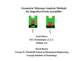
Geometric Tolerance Analysis Methods for Imperfect-Form Assemblies. Scott Pierce M.I. Technologies, L.L.C. Duluth, GA David Rosen George W. Woodruff School of Mechanical Engineering Georgia Institute of Technology. Outline. Introduction and Background Motivation

E N D
Geometric Tolerance Analysis Methods for Imperfect-Form Assemblies Scott Pierce M.I. Technologies, L.L.C. Duluth, GA David Rosen George W. Woodruff School of Mechanical Engineering Georgia Institute of Technology
Outline • Introduction and Background • Motivation • Our Approach: The Generate and Test Method • Development of the Tolerance Analysis Module • The Variational Modeling Environment • Simulation of Mating Between Imperfect-Form Components • Case Study • Conclusions and Future Work
Motivation A Very Simple Example: Two Squares in a Slot • The principal objective of this research is the development of a new, computer-aided approach to tolerance analysis • The purpose of tolerance analysis is to define the relationships between tolerance values, product functionality and manufacturing cost • In particular, we are interested in analysis of geometric tolerances that control form and orientation
Motivation A More Complex Example: The High-Speed Stapling Mechanism • A compound slider mechanism composed of several components • Multiple mating surfaces • Alignment between the driver, bender and bonnet affects functionality of the mechanism • Manufacturer has quality assurance data and process experience that define “typical manufacturing errors” How can the experience-based process knowledge be incorporated into this complex tolerance analysis problem?
Our Approach: Generate-and-Test Step 1: Generate “As Manufactured” Component Models
Our Approach: Generate-and-Test Step 2: Test the Effects of Manufacturing Errors by Simulating Mating Between As-Manufactured Components and Measuring Attributes of Functionality
Our Approach: Generate-and-Test • This Generate-and-Test Process is Repeated for a Series of Error Geometries and Magnitudes That are Representative of the Proposed Manufacturing Processes • Information Gained from this Analysis is Used to Guide the Tolerance Selection Process
Development of the Tolerance Analysis Module • The Variational Modeling Environment • Simulation of Mating Between Imperfect-Form Components
The Variational Modeling Environment • We have built a CAD environment that uses a NURBS surface representation to construct models of imperfect-form variants of prismatic components • The ACIS geometry engine is used as the modeling core • Constructed as a set of C++ classes and extensions to the ACIS api’s • Basic capabilities of the modeling environment allow: • Creation of prismatic parts • Use of Boolean operations to generate more complex prismatic geometry • Application of rigid-body transformations
The Variational Modeling Environment • Variational modeling capabilities allow: • Definition of pointset classes that define variant surfaces • Fitting of NURBS surfaces to a pointset to within a specified fitting tolerance. • Replacing nominally planar faces of prismatic components with variant NURBS surfaces.
The Variational Modeling Environment Verification: The Variational Modeling Module supports modeling of as-manufactured component variants to a resolution that is significant to tolerance analysis. Typical machining errors for end milling are on the order of 0.01 mm.
Simulation of Mating Between Imperfect-Form Components • Simulation of mating between surfaces that can be represented analytically is a well understood problem. • Simulation of mating between non-analytic, freeform surfaces is a much more difficult problem. Following a formulation originally proposed by Turner, we have chosen to formulate the mating problem as a mathematical programming problem of the form: • Minimize Z = total distance from perfect fit • s.t. non-interference between components
Simulation of Mating Between Imperfect-Form Components • How should “perfect fit” be defined? • For perfect-form, planar surfaces perfect fit means that faces are coplanar and that outward-facing normal vectors point in opposite directions. • Coplanarity implies that the distance between any point on one surface and the corresponding closest point on the other surface is zero. • This leads to the idea that for imperfect-form surfaces we should try to minimize the distance between any point on one surface and the corresponding closest point on the other surface
Non-Mating But Potentially Interfering Pair Mating Pair Mating Pair Simulation of Mating Between Imperfect-Form Components • We have chosen to use sampling grids to perform distance measurements and interference detection between surfaces • We find that the use of sampling grids is much more computationally efficient than the use of Boolean intersections • Grid density can be adjusted so that the resolution is fine enough to represent any significant surface feature.
Non-Mating But Potentially Interfering Pair Mating Pair Mating Pair Simulation of Mating Between Imperfect-Form Components Using this sampling grid approach, we can formulate the mating problem as a constrained optimization problem: Find: = (roll, pitch, yaw, x, y, z) = six degrees of freedom of the movable body. M = number of mating face pairs N = total number of mating face pairs, both mating and potentially interfering mF = number of gridpoints in the u-parameter direction for the given face pair nF = number of gridpoints in the v-parameter direction for the given face pair = minimum signed distance from gridpoint ij to the mating surface. F = 1…N, i = 1…mF, j = 1…nF
Grid Point Closest Point on Mating Surface Simulation of Mating Between Imperfect-Form Components • Selection of a Solution Method: • Finding the minimum distance between a grid point and the mating surface requires the solution of a point-projection problem • Point projections are the most computationally-intensive part of the mating simulation
Simulation of Mating Between Imperfect-Form Components Selection of a solution method (continued): We used published measurements of end-milled surfaces to generate test surfaces We explored the topography of the solution space generated by mating these surfaces We found the solution space to be nonlinear We found the boundaries of the feasible region to be nonlinear and in some cases non-convex
Simulation of Mating Between Imperfect-Form Components • We examined several potential solution methods including: • Successive linearization: • We have shown that both the objective and the constraints are highly nonlinear. Successive linearization will generally not converge well under these conditions • Generalized reduced gradient methods • Capable of handling nonlinear problems • Requires solution of a prohibitively large number of point projection problems
Simulation of Mating Between Imperfect-Form Components • We have chosen to modify the formulation of the mating problem to use the penalty function approach: where: WF = mating/non-mating face switch WINT = interference weighting factor (=100) The penalty function formulation converts the constrained formulation into an unconstrained problem, allowing the use of unconstrained optimization algorithms
Simulation of Mating Between Imperfect-Form Components To test potential solution algorithms we used two test problems: End-milling cutter deflection with four different surfaces “Correct” objective = 0.1484 End-milling cutter deflection with perfect-fit
Simulation of Mating Between Imperfect-Form Components • We tested three different solution algorithms for use with the penalty-function formulation: • Method 1: Simulated Annealing With Downhill Simplex: • Analogous to an annealing process, there is a finite probability of accepting an “uphill” move • This probability is reduced as the “temperature” is reduced • In theory, allows a more thorough search of the solution space so that local minima are avoided Where Z2 > Z1 In tests where we purposely introduced local minima into the solution space, simulated annealing was not very successful in avoiding them.
Simulation of Mating Between Imperfect-Form Components • Method 2: Randomized Hooke-Jeeves pattern search • Direct search method does not require the calculation of numerical gradients • Explores the region around a test point for the steepest descent direction, then moves in that direction until descent stops • When a downhill move cannot be found the step size is reduced and the exploration is repeated • Very robust in the presence of nonlinearities
Simulation of Mating Between Imperfect-Form Components • Method 3: Quasi-Newton Method • Gradient-based method • Uses a quadratic approximation to the objective function • Use first-order information to approximate the Hessian • Use line searches to generate the step size • We use the Broyden-Fletcher-Goldfarb-Shanno form of the quasi-Newton method. • We used a line search that starts with a quadratic approximation, then reverts to a golden section search when convergence slows.
Simulated Annealing Hooke-Jeeves BFGS Simulation of Mating Between Imperfect-Form Components Correct Answer: Objective = 0.1484 Best Answer from This Test: BFGS Objective = 0.1484 Convergence of all three solution methods for the four surface cutter deflection example
Simulated Annealing Hooke-Jeeves BFGS Simulation of Mating Between Imperfect-Form Components Convergence of all three solution methods for the perfect-fit cutter deflection example (correct objective value = 0)
Hooke-Jeeves Algorithm Alone Hybrid Algorithm When BFGS is Active Hybrid Algorithm After “Fallback” to Hooke-Jeeves BFGS Algorithm Alone Simulation of Mating Between Imperfect-Form Components Use of the hybrid BFGS/Hooke-Jeeves algorithm for the perfect-fit problem (correct objective value = 0)
Tolerance Analysis Module - Summary • Allows construction and manipulation of “as-manufactured” variant models • Simulates assembly of imperfect-form component variants • We now have a testbed that can be used to demonstrate the generate-and-test approach to tolerance analysis
Case Study • The case study is built upon a simplified version of the high-speed stapling mechanism • The components that have the most influence on the quality of the stapling process are included in the study: • Driver • Bender • Bonnet
Case Study Attribute of Functionality - Z-axis Rotation Z-Axis Rotation Attribute: Maximum possible difference between bender Z-rotation and driver Z-rotation Functional Limit: If Z-axis rotation exceeds 1.7 mrad the staple will buckle
Case Study In order to control the attributes of functionality we assign geometric tolerances of form and orientation: Bender What tolerance values should be assigned in order to ensure that the mechanism will function?
Case Study • Step 1: Group the surfaces of the stapling mechanism into four groups • All surfaces within a group would be manufactured in a single setup, therefore they share a common level of precision
Case Study • Step 2: Generate “as-manufactured” models of higher precision (higher cost) and lower precision (lower cost) variants of each surface group • All error data comes from published measurements or results of end-milling simulations.
Case Study • Step 2 (continued): • Each component variant was measured using a functional gauging routine • The results of each measurement were the tolerance values that the particular variant would meet
Case Study • Mating simulation was performed for every combination of higher/lower precision surface groups • The mechanism components were mated at a series of positions through the stapling process • Functional attributes were measured • The results were used to construct a 24 full-factorial analysis for each functional attribute
Case Study Analysis of Variance for the Z-axis rotation attribute: Significant effects: Bender Groove, Bonnet Setting both of these surface groups to higher precision results in a maximum Z-axis rotation of 1.92 mrad. This is still above the functional limit of 1.7mrad, so the tolerance on the bender groove needs to be tightened further if possible
Case Study Combining the results of the Z-axis rotation study with results from a study on a second functional attribute, we selected geometric tolerance values that strike a balance between the need for precision and manufacturing cost.
Conclusions • I have described the development of an environment for computer-aided tolerance analysis. • Allows the inclusion of experience-based manufacturing information through the use of the generate-and-test method of tolerance analysis. • Development of an effective algorithm for simulation of mating between imperfect-form, non-analytic surfaces was key to the generate-and-test method. • Through the case study, I have shown that this method can be used as an aid in the selection of geometric tolerances of form and orientation.
Possibilities for Future Work • Link mating simulation with a kinematic analysis in order to bring force balance information into the picture. • Extend to non-prismatic geometry. • Apply the non-analytic surface mating methods in areas other than tolerance analysis (e.g. design of components whose perfect-form geometry is non-analytic).