Optimization Techniques in Applied Mathematics: Understanding Linear and Mixed Integer Programming
430 likes | 668 Views
This lecture delves into optimization principles in applied mathematics, focusing on formulating and solving optimization problems. It covers linear programming (LP) and mixed-integer linear programming (MILP), exploring practical examples such as production scheduling and cost minimization. Key concepts such as objective functions, constraints, and feasible sets are introduced, providing a comprehensive understanding of optimization strategies. Real-world applications demonstrate the significance of optimization in improving efficiency across various industries.

Optimization Techniques in Applied Mathematics: Understanding Linear and Mixed Integer Programming
E N D
Presentation Transcript
System Planning 2013 • Lecture 7: Optimization • Appendix A • Contents: • General about optimization • Formulating optimization problems • Linear Programming (LP) • Mixed Integer Linear Programming (MILP)
Optimization – General • Discipline in applied mathematics • Used when: • Want to maximize or minimize something (e.g. profit or cost) under various conditions (e.g. generation capacities, transmission limits)
Optimization – General Typical problems • In what sequence should parts be produced on a machine in order to minimize the change-over time? • How can a dress manufacturer lay out its patterns on rolls of cloth to minimize wasted material? • How many elevators should be installed in a new office building to achieve an acceptable expected waiting time? • What is the lowest-cost formula for chicken food which will provide required quantities of necessary minerals and other nutrients? • What is the generation plan for the power plants during the next six hours?
Defines the feasible set Optimization - General The general optimization problem: • f(x): objective function • x: optimization variables (vector) • g(x),h(x):constraints (vectors) • and : variabel limits (vector)
Optimization – Formulation Formulation of optimization problems: • Describe the problem in words: • Think through the problem • Define symbols • Review the parameters and variables involved • Write the problem mathematically • Translate the problem defined in words to mathematics
? Optimization – Formulation The problem: A manufacturer owns a number of factories. How should the manufacturer ship his goods to the customers?
Optimization – Formulation • The factories cannot produce more than their production capacities. • The customers must at least receive their demand • The problem in words:How should the merchandise be shipped in order to minimize the transportation costs? The following must be fulfilled:
Optimization – Formulation 2. Define symbols: • Index and parameters: • m factories, factory i has capacity ai • n customers, customer j demand bj units of the commodity • The transportation cost from factory i to customer j is cij per unit • Variables • Let xij, i = 1...m, j = 1...n denote the number of units of the commodity shipped from factory i to customer j
Optimization – Formulation 3. Mathematical formulation: • Objective function • Transportation cost: • Constraints • Production capacity: • Demand: • Variable limits:
Optimization – Formulation The optimization problem:
LP – General Linear Programming problems (LP problems) • Class of optimization problems with linear objective function and constraints • All LP problems can be written as (standard form):
LP – General • LP problems will here be explained through examples (similar as in Appendix A) • Will have to look at the following: • Extreme points • Slack variables • Non existing solution • Not active constraints • No finite solution or unbounded problems • Degenerated solution • Flat optimum • Duality • Solution methods
LP – Example • The problem:
x 2 4 z = 40 3 z = 30 z = 20 2 1 x2 0 x x1 0 1 1 2 3 4 4x1+12x2 12 x1+x2 2 LP – Example Optimum in: Objective:
x 2 4 z = 40 3 z = 30 z = 20 2 1 x2 0 x x1 0 1 1 2 3 4 4x1+12x2 12 x1+x2 2 LP – Extreme points • The “corners” of the feasible set are called extreme points • Optimum is always reached in one or more extreme points!
LP – Slack variables • LP problem on standard form: • Introduce slack variables in order to write inequality constraints using equality
LP – Slack variables • Without slack variables:(Ax b) • With slack variables: (Ax = b)
New constraint LP – Non existing solution • Can happen that the constraints makes no solution feasible! (Bad formulation of problem)
x 2 4 A: Feasible set defined by (a) & (b) 3 2 x1+x2 1 (c) 1 x2 0 B: Feasible set defined by (c) x x1 0 1 1 2 3 4 4x1+12x2 12 x1+x2 2 LP – Non existing solution Feasible set is empty! (b) (a)
LP – Not active constraints • Some constraints might not be active in optimum. New constraint
Not active constraints x1+x2 7 Active constraints LP – Not active constraints x 2 4 z = 40 3 z = 30 z = 20 2 1 x2 0 x x1 0 1 1 2 3 4 4x1+12x2 12 x1+x2 2
LP – No finite solution • If the constraints don’t limit the objective: |z| New objective function
z = -5 z = -4 z = -3 LP – No finite solution x 2 4 min z - 3 2 1 x2 0 x 1 1 2 3 4 x1 0 4x1+12x2 12 x1+x2 2
LP – Degenerated solution • More than one extreme point can be optimal. All linear combinations of these points are then also optimal New objective
z = 50 z = 40 z = 30 LP – Degenerated solution x 2 The line between the extreme points are also optimal solutions 4 3 2 1 x2 0 x x1 0 1 1 2 3 4 4x1+12x2 12 x1+x2 2
LP – Flat optimum • A number of extreme points can have almost the same objective function value. New objective
z = 19.980 z = 19.995 LP – Flat optimum x 2 4 z = 50 z = 40 3 z = 30 2 1 x2 0 x x1 0 1 1 2 3 4 4x1+12x2 12 x1+x2 2
LP – Duality • All LP problems (primal problem) have a corresponding dual problem • are called dual variables Dual problem: Primal problem:
LP – Duality Theorem (strong duality): If the primal problem has an optimal solution, then also the dual problem has an optimal solution and the objective values of these solutions are the same.
LP – Duality • Q: What does the dual variables describe? • A: Dual variables = Marginal value of the constraint that the dual variable represents, i.e. how the objective function value changes when the right-hand side of the constraint changes One dual variable for each constraint!
3 x1+x2 7 LP – Duality x 2 4 z = 40 3 z = 30 z = 20 2 In optimum: 1 > 0 (active) 2 > 0 (active) 3 = 0 (not active) 1 x2 0 x x1 0 1 1 2 3 4 4x1+12x2 12 x1+x2 2 2 1
LP – Duality • Dual variables • Small changes in right-hand side b • Change in objective function value z: z = Tb
MILP – General • Mixed Integer Linear Programming problems (MILP problems) • Class of optimization problems with linear objective function and constraints • Some variables can only take integer values
x 2 4 z = 40 3 z = 30 z = 20 2 1 x2 0 x x1 0 1 1 2 3 4 4x1+12x2 12 x1+x2 2 MILP – Example Optimum in: Objective:
MILP – Solving • Easy to implement integer variables. • Hard to solve the problems. • Execution times can increase exponentially with the number of integer variables • Avoid integer variables if possible! • Special case of integer variables: Binary variables x {0,1}
x2 x1 MILP – Example • Minimize the cost for buying ”something” • Variable, x: Quantity of ”something”, x 0. • Not constant cost per unit - cost function. • For example: Discount when buying more than a specified quantity: Cost [SEK] Split x into two different variables, x1 and x2. Observe that x1≤ xb. Also note that both x1 and x2 are 0. Number of ”units” xb
Cost [SEK] x2 x1 Number of ”units” xb MILP – Example • Cheaper to buy in segment 2 Must force the problem to fill the first segment before entering segment 2. • Can be performed by introducing a binary variable.
Cost [SEK] x2 x1 Number of ”units” xb Check if s=0: Check if s=1: MILP – Example • Introduce the following constraints: • Let s be an integer variable indicating whether being in segment 1 or 2. s=0 s=1 where M is an arbitrarely large number.
LP – Solution methods • Simplex: • Returns optimum in extreme point (also when • degenerated solution) • Interior point methods: • If degenerated solution: Returns solution between two • extreme points
Simplex Interior point method LP – Solution methods x 2 4 z = 50 z = 40 3 z = 30 2 1 x2 0 x1 0 1 2 3 4 4x1+12x2 12 x1+x2 2
PROBLEM 11 - Solutions to LP problems Assume that readymade software is used to solve an LP problem. In which of the following cases do you get an optimal solution to the LP problem and in which cases do you have to reformulate the problem (or correct an error in the code). a) The problem has no feasible solution. b) The problem is degenerated. c) The problem does not have a finite solution.