Download
1 / 54
540 likes | 648 Views
Learn about Insertion sort, Heapsort, Mergesort & Quicksort algorithms for efficient sorting. Dive into analysis, memory usage, and practical examples.

E N D
G64ADSAdvanced Data Structures Sorting
Insertion sort 1) Initially p = 1 2) Let the first p elements be sorted. 3) Insert the (p+1)th element properly in the list so that now p+1 elements are sorted. 4) increment p and go to step (3)
Insertion sort Consists of N - 1 passes For pass p = 1 through N - 1, ensures that the elements in positions 0 through p are in sorted order elements in positions 0 through p - 1 are already sorted move the element in position p left until its correct place is found among the first p + 1 elements 4
Insertion sort To sort the following numbers in increasing order: 34 8 64 51 32 21 p = 1; tmp = 8; 34 > tmp, so second element a[1] is set to 34: {8, 34}… We have reached the front of the list. Thus, 1st position a[0] = tmp=8 After 1st pass: 8 34 64 51 32 21 (first 2 elements are sorted) 5
p = 2; tmp = 64; 34 < 64, so stop at 3rd position and set 3rd position = 64 After 2nd pass: 8 34 64 51 32 21 (first 3 elements are sorted) p = 3; tmp = 51; 51 < 64, so we have 8 34 64 64 32 21, 34 < 51, so stop at 2nd position, set 3rd position = tmp, After 3rd pass: 8 34 51 64 32 21 (first 4 elements are sorted) p = 4; tmp = 32, 32 < 64, so 8 34 51 64 64 21, 32 < 51, so 8 34 51 51 64 21, next 32 < 34, so 8 34 34, 51 64 21, next 32 > 8, so stop at 1st position and set 2nd position = 32, After 4th pass: 8 32 34 51 64 21 p = 5; tmp = 21, . . . After 5th pass: 8 21 32 34 51 64 6
Insertion sort: worst-case running time Inner loop is executed p times, for each p=1..N-1 Overall: 1 + 2 + 3 + . . . + N-1 = …= O(N2) Space requirement is O(?) 7
Heapsort (1) Build a binary heap of N elements the minimum element is at the top of the heap (2) Perform N DeleteMin operations the elements are extracted in sorted order (3) Record these elements in a second array and then copy the array back 8
Heapsort -Analysis (1) Build a binary heap of N elements repeatedly insert N elements O(N log N) time (2) Perform N DeleteMin operations Each DeleteMin operation takes O(log N) O(N log N) (3) Record these elements in a second array and then copy the array back O(N) Total time complexity: O(N log N) Memory requirement: uses an extra array, O(N) 9
Heapsort – No Extra Memory Observation: after each deleteMin, the size of heap shrinks by 1 We can use the last cell just freed up to store the element that was just deleted after the last deleteMin, the array will contain the elements in decreasing sorted order To sort the elements in the decreasing order, use a min heap To sort the elements in the increasing order, use a max heap the parent has a larger element than the child 10
Heapsort – No Extra Memory Sort in increasing order: use max heap Delete 97 11
Mergesort Based on divide-and-conquer strategy Divide the list into two smaller lists of about equal sizes Sort each smaller list recursively Merge the two sorted lists to get one sorted list How to divide the list Running time How to merge the two sorted lists Running time 12
Mergesort Based on divide-and-conquer strategy Divide the list into two smaller lists of about equal sizes Sort each smaller list recursively Merge the two sorted lists to get one sorted list How to divide the list Running time How to merge the two sorted lists Running time 13
Mergesort: Divide If the input list is a linked list, dividing takes (N) time We scan the linked list, stop at the N/2 th entry and cut the link If the input list is an array A[0..N-1]: dividing takes O(1) time we can represent a sublist by two integers left and right: to divide A[left..right], we compute center=(left+right)/2 and obtain A[left..center] and A[center+1..right] Try left=0, right = 50, center=? 14
Mergesort Divide-and-conquer strategy recursively mergesort the first half and the second half merge the two sorted halves together 15
Mergesort 16
Mergesort: Merge Input: two sorted array A and B Output: an output sorted array C Three counters: Actr, Bctr, and Cctr initially set to the beginning of their respective arrays (1) The smaller of A[Actr] and B[Bctr] is copied to the next entry in C, and the appropriate counters are advanced (2) When either input list is exhausted, the remainder of the other list is copied to C 17
Mergesort: Analysis Merge takes O(m1 + m2) where m1 and m2 are the sizes of the two sublists. Space requirement: merging two sorted lists requires linear extra memory additional work to copy to the temporary array and back 20
Mergesort: Analysis Let T(N) denote the worst-case running time of mergesort to sort N numbers. Assume that N is a power of 2. Divide step: O(1) time Conquer step: 2 T(N/2) time Combine step: O(N) time Recurrence equation: T(1) = 1 T(N) = 2T(N/2) + N 21
Mergesort: Analysis Since N=2k, we have k=log2 n 22
Quicksort Divide-and-conquer approach to sorting Like MergeSort, except Don’t divide the array in half Partition the array based elements being less than or greater than some element of the array (the pivot) Worst case running time O(N2) Average case running time O(N log N) Fastest generic sorting algorithm in practice Even faster if use simple sort (e.g., InsertionSort) when array is small 23
Quicksort Algorithm Given array S Modify S so elements in increasing order If size of S is 0 or 1, return Pick any element v in S as the pivot Partition S – {v} into two disjoint groups S1 = {x Є(S –{v}) | x ≤ v} S2 = {x Є(S –{v}) | x ≥ v} Return QuickSort(S1), followed by v, followed by QuickSort(S2) 24
Why so fast? MergeSort always divides array in half QuickSort might divide array into subproblems of size 1 and N-1 When? Leading to O(N2) performance Need to choose pivot wisely (but efficiently) MergeSort requires temporary array for merge step QuickSort can partition the array in place This more than makes up for bad pivot choices 26
Picking the Pivot Choosing the first element What if array already or nearly sorted? Good for random array Choose random pivot Good in practice if truly random Still possible to get some bad choices Requires execution of random number generator 27
Picking the Pivot Best choice of pivot? Median of array Median is expensive to calculate Estimate median as the median of three elements Choose first, middle and last elements e.g., <8, 1, 4, 9, 6, 3, 5, 2, 7, 0> Has been shown to reduce running time (comparisons) by 14% 28
Partitioning Strategy Partitioning is conceptually straightforward, but easy to do inefficiently Good strategy Swap pivot with last element S[right] Set i = left Set j = (right –1) While (i < j) Increment i until S[i] > pivot Decrement j until S[j] < pivot If (i < j), then swap S[i] and S[j] Swap pivot and S[i] 29
Partitioning Strategy How to handle duplicates? Consider the case where all elements are equal Current approach: Skip over elements equal to pivot No swaps (good) But then i = (right –1) and array partitioned into N-1 and 1 elements Worst case O(N2) performance 32
Partitioning Strategy How to handle duplicates? Alternative approach Don’t skip elements equal to pivot Increment i while S[i] < pivot Decrement j while S[j] > pivot Adds some unnecessary swaps But results in perfect partitioning for array of identical elements Unlikely for input array, but more likely for recursive calls to QuickSort 33
Small Arrays When S is small, generating lots of recursive calls on small sub-arrays is expensive General strategy When N < threshold, use a sort more efficient for small arrays (e.g., InsertionSort) Good thresholds range from 5 to 20 Also avoids issue with finding median-of-three pivot for array of size 2 or less Has been shown to reduce running time by 15% 34
Analysis of QuickSort Let i be the number of elements sent to the left partition Compute running time T(N) for array of size N T(0) = T(1) = O(1) T(N) = T(i) + T(N –i –1) + O(N) 38
Lower Bound on Sorting Best worst-case sorting algorithm (so far) is O(N log N) Can we do better? Can we prove a lower bound on the sorting problem? Preview For comparison sorting, no, we can’t do better Can show lower bound of Ω(N log N) 44
Decision Trees A decision tree is a binary tree Each node represents a set of possible orderings of the array elements Each branch represents an outcome of a particular comparison Each leaf of the decision tree represents a particular ordering of the original array elements 45
Decision Tree for Sorting The logic of every sorting algorithm that uses comparisons can be represented by a decision tree In the worst case, the number of comparisons used by the algorithm equals the depth of the deepest leaf In the average case, the number of comparisons is the average of the depths of all leaves There are N! different orderings of N elements 47
Lower Bound for Comparison Sorting Lemma 7.1 Lemma 7.2 Theorem 7.6 Theorem 7.7 48
Linear Sorting Some constraints on input array allow faster than Θ(N log N) sorting (no comparisons) CountingSort Given array A of N integer elements, each less than M Create array C of size M, where C[i] is the number of i’s in A Use C to place elements into new sorted array B Running time Θ(N+M) = Θ(N) if M = Θ(N) 49
Linear Sorting BucketSort Assume N elements of A uniformly distributed over the range [0,1) Create N equal-sized buckets over [0,1) Add each element of A into appropriate bucket Sort each bucket (e.g., with InsertionSort) Return concatentation of buckets Average case running time Θ(N) Assumes each bucket will contain Θ(1) elements 50