Download
1 / 17
170 likes | 194 Views
A numerical simulation study on helioseismology with harmonic and non-harmonic sources in the solar subphotosphere. Investigating wave propagation features and convective instability effects.

E N D
Acoustic wave propagation in the solar subphotosphere S. Shelyag, R. Erdélyi, M.J. Thompson Solar Physics and upper Atmosphere Research Group, Department of Applied Mathematics, University of Sheffield, Sheffield, UK
Outline We aim to develop a numerical “toolbox” for helioseismological studies • Numerical setup • Harmonic source • Local cooling event (non-harmonic source) • Some analysis
The simulation setup Full 2-dimensional HD Cartesian geometry Total Variation Diminishing spatial discretization scheme Fourth order Runge-Kutta time discretization The simulation domain: 150 Mm wide and 52.6 Mm deep, 600x4000 grid points The upper boundary of the domain is near the temperature minimum Two boundary regions of 1.3 Mm each at the top and bottom boundaries The main part of the domain is 50 Mm deep
The simulation domain We look at the level ~600 km below the upper boundary The source is located ~200 km below this level
The model profile temperature density convection <0: no >0: yes sound speed Modified Christensen-Dalsgaard's standard Model, pressure equilibrium.
Convective instability Convective instability is suppressed: 1=const=5/3 This approach has advantage, because the waves, while propagating throughthe quiescent medium, can be observed more clearly, undisturbed by convective fluid motions far from the source.
Source #1 Harmonic pressure perturbation (cf. Tong et al. 2003): p is the pressure perturbation amplitude t – real time T=5.5 min
Evolution of pressure perturbation #1 Consecutive snapshots of pressure deviation p in the simulated domain after the harmonic perturbation has been introduced. High order acoustic modes produced by interference of the lower ones can be noticed in the upper part of the domain on the latest snapshots.
Time-distance diagram #1 Synthetic time-distance diagram (the cut of p/p0 is taken at about 600 kmbelow the upper boundary of the domain).
Source #2 Localized cooling event causing local convective instability, mass inflow and sound waves extinction where timescale 1=120 s Power spectrum of the source
Velocity field around the source The behavior of the source in time can be understood as two stages. In the beginning, the source creates expanding inflow and the pressure and temperature drop. At the second stage, due to an increased temperature gradient, two convective cells surrounding the source are developed.
Time-distance diagram #2 Time-distance diagram produced with the non-harmonic source. The picture is covered by the flows caused by the source.
Time-distance diagram #2 Pressure cut with high-pass frequency filtering applied. The filtering revealed seismic traces similar to the ones shown for the harmonic source.
Single non-harmonic source, some analysis The power spectrum of the time-distance diagram generated by a single perturbation source. The p-modes are visible up to high orders. The theoretically calculated p1mode is marked by two dashed lines.
Multiple non-harmonic sources, some analysis The power spectrum of a large number of sources randomly distributed along a selected depth and time. The features, connected with fluid motions caused by these sources, and the high order p-modes faint with the growth of the number of random sources. The p1mode is marked in the same way as before.
To-do list • Better boundaries are necessary • Non-uniform grid (and possibility of 3D) • Magnetic field