Download
1 / 123
1.23k likes | 1.35k Views
Fast Image Search. Presented by:. Uri Shabi Shiri Chechik. For the Advanced Topics in Computer Vision course Spring 2007. Introduction. - The tasks. Recognition :

E N D
Fast Image Search Presented by: Uri Shabi Shiri Chechik For the Advanced Topics in Computer Vision course Spring 2007
Introduction - The tasks Recognition: • Given a database of images and an input query image, we wish to find an image in the database that represents the same object as in the query image. Classification: • Given a database of images, the algorithm: • Divides the images into groups • Given a query image it returns the group that the image belongs to
Introduction - The tasks Database Query Image Results D Nister, H Stewenius. Scalable Recognition with a Vocabulary Tree. CVPR’06. 2006.
Introduction - The tasks Database Query Image
Introduction - The problem D Nister, H Stewenius. Scalable Recognition with a Vocabulary Tree. CVPR’06. 2006.
Introduction - How many object categories are there? Biederman 1987
Introduction - The Challenges Challenges 1: view point variation Michelangelo 1475-1564 Adapted with permission from Fei Fei Li - http://people.csail.mit.edu/torralba/iccv2005/
Introduction - The Challenges Challenges 2: illumination Adapted with permission from Fei Fei Li - http://people.csail.mit.edu/torralba/iccv2005/
Introduction - The Challenges Challenges 3: occlusion Magritte, 1957 Adapted with permission from Fei Fei Li - http://people.csail.mit.edu/torralba/iccv2005/
Introduction - The Challenges Challenges 4: scale Adapted with permission from Fei Fei Li - http://people.csail.mit.edu/torralba/iccv2005/
Introduction - The Challenges Challenges 5: deformation Xu, Beihong 1943 Adapted with permission from Fei Fei Li - http://people.csail.mit.edu/torralba/iccv2005/
Introduction - The Challenges To sum up, we have few challenges: • View point variation • Illumination • Occlusion • Scale • Deformation
Introduction - Bag of Words (Documents) • A document can be represented by a collection of words • Common words can be ignored (the, an,etc.) – This is called a ‘stop List’ • Words are represented by their stems • ‘walk’, ‘walking’, ‘walks’ ’walk’ • A topic can be recognized by Word frequencies Sivic & Zisserman. Video Google: a text retrieval approach to object matching in videos, Computer Vision, 2003
sensory, brain, visual, perception, retinal, cerebral cortex, eye, cell, optical, eye nerve, image, visual, Hubel, Wiesel Introduction - Bag of Words (Documents) Analogy to documents Of all the sensory impressions proceeding to the brain, the visual experiences are the dominant ones. Our perception of the world around us is based essentially on the messages that reach the brain from our eyes. For a long time it was thought that the retinal image was transmitted point by point to visual centers in the brain; the cerebral cortex was a movie screen, so to speak, upon which the image in the eye was projected. Through the discoveries of Hubel and Wiesel we now know that behind the origin of the visual perception in the brain there is a considerably more complicated course of events. By following the visual impulses along their path to the various cell layers of the optical cortex, Hubel and Wiesel have been able to demonstrate that the message about the image falling on the retina undergoes a step-wise analysis in a system of nerve cells stored in columns. In this system each cell has its specific function and is responsible for a specific detail in the pattern of the retinal image. sensory perception Visual X 2 brain retinal cerebral image cell eye X 2
Introduction - Bag of Words • Images can be represented by visual words • An object in an image can be recognized by visual word frequencies J Sivic, A Zisserman. Video Google: a text retrieval approach to object matching in videos. Computer Vision, 2003.
Introduction - Visual word • We could use a feature as a visual word, but • Too many features • Two features of the same object will never look the same • A visual word is a “visual stem” which is represented by a descriptor • What is a good code word (visual word)? • Invariant to different view points, illumination, scale, shift and transformation
Object Bag of ‘words’ Introduction - Bag of Words Adapted with permission from Fei Fei Li - http://people.csail.mit.edu/torralba/iccv2005/
Adapted with permission from Fei Fei Li - http://people.csail.mit.edu/torralba/iccv2005/
Introduction - Bag of Words • The fact that we only use the frequencies of visual words, implies that this method is Translation Invariant. • This is why it is called a ‘Bag of Words’, since two images with the same words are identified as the same image
Breaking down the problem • Feature Detection • Feature Description • Feature Recognition – how to find similar words to a query feature from a database of code words • Image Recognition\Classification – how to find similar images to the query image\ how to classify our image
learning recognition codewords dictionary Feature detection & representation image representation Image recognition category models (and/or) classifiers Adapted with permission from Fei Fei Li - http://people.csail.mit.edu/torralba/iccv2005/
Feature Detection • We can use any feature detection algorithms • We can use a mixture of feature detections and capture more types of features • What is a good detection? • Invariant to rotation, illumination, scale, shift and transformation
Feature Description • What is a good descriptor? • Invariant to different view points, illumination, scale, shift and transformation • The image recognition is rotation or scale invariant if the detector & descriptor are as well.
Feature Description • SIFT descriptor • Local Frames of Reference
Feature Description - SIFT • We determine a local orientation according to the dominant gradient • Define native coordinate system • We take a 16×16 window and divide it into 16 4×4 windows • We then compute the gradient orientation histogram of 8 main directions for each window
Feature Description - SIFT • Properties • Rotation invariant
Feature Description - Local Affine Frames of Reference • Works together with Distinguished Regions detector • Assumption: Two frames of the same objects are related by affine transformation • Idea: Find an affine transformation that best normalizes the frame. • Two normalized frames of the same object will looks similar Stˇep´an Obdrˇz´alek,Jirı Matas.Object Recognition using Local Affine Frames on Distinguished Region
Feature Description - Local Frames of Reference • Properties • Rotation invariant (depending on the shape) • Brings different features of the same object to be similar – A great advantage! Could test similarity of features with great efficiency
Feature Description - How to normalize? • In affine transformation we have 6 degrees of freedom, that can enforce 6 constraints • An example to the constraints: • Rotate the object around the line from the center of gravity to the most extreme point
Fast Feature Recognition A reminder: • Given a database of code words and a query feature, we find the closest code word to the feature Database Query Feature
Fast Feature Recognition - Inverted File • Each (visual) word is associated with a list of (images) documents containing it
Fast Feature Recognition - Inverted File • Each image in the database is scored according to how many common features it has with the query image. • The image with the best score is selected • Also note, that in order for the object to be recognized successfully (compete with background regions) it need to be large enough (at least ¼ of image area)
Fast Feature Recognition • Why do we need different approaches? • Why can’t we just use a table? • There could be too many visual words and we want a fast solution!
Fast Feature Recognition Three different approaches: • A small number of words • Vocabulary Tree • Decision Tree
Fast Feature Recognition - A small number of words Construction of the vocabulary: • We take a large training set of images from many categories • Then form a codebook containing W words using the K-means algorithm Recognition phase: • We sequentially find the nearest neighbor of the query feature R Fergus, L Fei-Fei, P Perona, A Zisserman. Learning Object Categories from Google’s Image Search. ICCV 2005.
Fast Feature Recognition - A small number of words
Fast Feature Recognition - A small number of words
Fast Feature Recognition - A small number of words Pros: • Going sequentially over the words leads high accuracy • Space efficiency - we save only a small number of words Cons: • A small number of words doesn’t capture all the features
A small Detour - K-Mean Clustering • Input • A set of n points {x1,x2,…,xn} in a d-dimensional feature space (the descriptors) • Number of clusters - K • Objective • To find the partition of the points into K non-empty disjointed subsets • So that each group consists of the descriptors closest to a particular center
A small Detour - K-Mean Clustering Step 1: • Randomly choose K equal size sets and calculate their centers m1
A small Detour - K-Mean Clustering Step 2: • For each xi: Assign xi to the cluster with the closest center
A small Detour - K-Mean Clustering Step 3: Repeat until “no update” • Compute the mean (mass center) for each cluster • For each xi: Assign xi to the cluster with the closest center
A small Detour - K-Mean Clustering • The final result:
Fast Feature Recognition - Vocabulary Tree Idea: • Use many visual words – capture all features • But since we can’t sequentially go over a large number of words we’ll use a tree! D Nister, H Stewenius. Scalable Recognition with a Vocabulary Tree. CVPR’06. 2006.
Fast Feature Recognition - Vocabulary Tree Construction of the vocabulary: • Input: A large set of descriptor vectors • Partition the training data into K groups, where each group consists of the descriptors closest to a particular center • Continue recursively for each group up to L levels Recognition phase: • Traverse the tree up to the “leaves” which will hopefully contain the closest word
Fast Feature Recognition - Vocabulary Tree
Fast Feature Recognition - Vocabulary Tree
Fast Feature Recognition - Vocabulary Tree
Fast Feature Recognition - Vocabulary Tree
Fast Feature Recognition - Vocabulary Tree