Download
1 / 23
240 likes | 555 Views
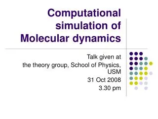
Computational simulation of Molecular dynamics. Talk given at the theory group, School of Physics, USM 31 Oct 2008 3.30 pm. Plan of the talk. Scope of investigation General idea and simulation strategy Simplest simulation: 2D, rigid boundary condition, without interaction

E N D
Computational simulation of Molecular dynamics Talk given at the theory group, School of Physics, USM 31 Oct 2008 3.30 pm
Plan of the talk • Scope of investigation • General idea and simulation strategy • Simplest simulation: 2D, rigid boundary condition, without interaction • Some details of Mathematica programming • Periodic boundary condition • Generalisation to 3D case, with interactions • Abstraction of physical quantities from the simulation (work still in progress)
General idea: Interactions determine physical behavior • Consider a system of particles interacting among themselves via some inter-particle forces arises from some effective potential. • Well known example of such potential are the Lennard –Jones potential (6-12 potential) of intermolecular force in Argon gas • VLJ = k(a/r6 – b/r12) • These forces determine the behaviour of the particle system – heat capacities, pressure, crystal structures, phase transition etc. • Different system is characterised by different interactions (different type of potential, parameters) • Once the exact form of interactions is identified, the physical consequences could be worked out either theoretically, or using computational methods.
Empirical interactions • The LJ potential is a so-called ‘empirical potential’ • Their 6-12 form is an educated ‘guess’ that fits experimental data of the system investigated (e.g. Argon and other inert gases) • The parameters in the LJ potential have to be extracted from experimental data • Not predicted from first principle • Different system has different values of a, b, k • System of different interactions may not be described by the LJ potential – other empirical form of potential is required.
System of particles • Main purpose: To predict the behaviour and extract essential physical observables of a system of interacting particles (given a known potential) at a given temperature. • The ‘particle’ could be entities with internal structures such as complex molecules, or simply a ‘point’ particle.
If temperature changes at t1 to T2, system will evolve to a new equilibrium state corresponds to T2 Total energy Equilibrium state corresponds to T1 Equilibrium state corresponds to T2 Initial configuration t2 t1 time Temperature fixed at T1 Temperature fixed at T2 System evolved as a function of time at a fixed temperature At a fixed temperature, the (i) evolution of the system from i to equilibrium and (ii) the energy of the equilibrium state is determined by the interactions among the particles (and possible external influences e.g. external magnetic or electric field, or pressure)
Tracing the evolution is possible – computational simulation • Essentially, the dynamical development as a function of time from some initial (non-equilibrium) state to a final (equilibrium) state can be traced in principle if the interactions are known. • Trace the evolution using computational methods.
First principle derivation of interaction • The potential or forces among the particles are quantum-mechanical in nature. • In principle these force can be derived from first-principle (ab-initio) by solving the many-body quantum-mechanical Schroedinger equation. • Then these forces are fed into a computer code to predict the behaviour of the system. • No experimental input is required in principle. • Parameter free. • Quantum-molecular dynamics – computationally expensive – further work. • Only classical, empirical molecular dynamics will be discussed.
Instantaneous informationof each particles • If we can trace (i) the instantaneous position and (ii) instantaneous velocities of each particle, as a function of time at a fixed temperature, we then can • (i) Abstract time averages of physical quantities (e.g. correlation length, heat capacities etc.) (ii) Known if phase transition has occured (iii) Display the motion of these particle on the computer screen (merely for visualisation purpose is possible) (iv) Many other things…
Simplest case: 2D free particle bouncing in a box • Imagine a 2-D box of size L x L, containing N free particles bouncing against the wall • Forces among the particle is F = 0 • How would you simulate their behavior and visually display them on the computer screen? • Essentially, we wish to (i) track instantaneous position, r(np)[n] and (ii) instantaneous velocities v(np)[n] • r(np)[n], v(np)[n] positional vector and velocity of particle indexed by np at the time step n.
Size of the box y = L r(np)[n] r(np=1)[n] r(np=2)[n] y = 0 x = L x = 0
Mathematica Simulationof rigid boundary box containing free particles
Algorithm • Initialisation: Number of particles, masses, positions, velocity • Need to make sure that the total momentum of the system is zero a trick is required: • Let mom[np] is the momentum of particle np, • Calculate the sum of all momentum, SumMom = Sum[mom[np],{np, 1, N}] • Divided SumMom by N give average momentum per particle, mom_ave • Then replace the mom[np] mom[np] – mom_ave • When sum over mom[np] for all np from 1 to N, we will be assured that SumMomentum
Kinematical equations of r • Evolve the particle’s position according to the kinematical relation r[np][n] = r[np][n-1] + v[np] deltat • v[np] is a constant in time for each particle since no interactions act on the particle to modify the velocity. • Loop the time step, n, from n=0 to n=nmax.
Problems with the simulation • Not physical • No interaction • Box size is too small • Number of particle is too small • Computer hangs if N1023, L~ m • Edge effect: Bouncing at edges is significant whereas for real cases it is otherwise for real case value of L, N In real case, L ~ m, N~1023
Computational tricks to circumvent edge effect • Force ignored for the moment (take care of it later) • Use periodic boundary condition: • If x > L, x (x - L) • If x < 0, x (x +L) • This trick essentially eliminates the bouncing boundary effects at the edges – artificial simulation of an ‘infinite’ volume
Mathematica Simulationof a box containing free particles with periodic boundary condition
Trick to simulate large number of particle: Kaleidoscoping • Problem still exist to simulate large N • The trick: Kaleidoscoping 8 cell surrounding the central cell to simulate the presence of other particles (which are mirror image of the ones in the central cell) • Keleidoscoping creates a total of 9N evolving particles despite only N are actually involved in the kinematical time-stepping • “fake” reality approximates true reality by using larger N • Needed if forces are taken into account later • Save computational resources: get 9N particles in the picture despite only evolve N of them (for 2D case) • Can generalise to 3D case easily Keleidoscoping 26 cells surrounding the central cell get 27N particles in the picture despite only evolve N of them
Mathematica Simulationof kelediasoped box containing free particles
May the force be with you… • Forces among the particle is switched on no more r[np][n] = r[np][n-1] + v[np] deltat • Force between them can be then numerically evaluated via Fr = - dV(r)/dr if the form of the potentialV(r) between two particles with r[np1] and r[np2] are known • VLJ = k(a/r6 – b/r12) • Let DR =|r[np1]- r[np2]| ( r in VLJ) • Fr = - k( -6a / DR7 + 12 b/DR13) • The evolution of kinematical coordinates can be derived from Newton second law Verlet algorithm
Verlet algorithm Next n
Mathematica Simulationof kelediasoped box containing interacting particles
Work to be done • It’s a project still in progress. • The evolution from initial state to equilibrium state has at fixed temperature is yet to carry out • Abstraction of physical information such as heat capacity, transport coefficients is yet to be done • Investigation of phase transition will be possible since the critical parameters can be numerically obtained • Incooperating some internal degree of freedom into the ‘particle’, simulation of structural phase transition of liquid crystal is possible.