Balanced Trees

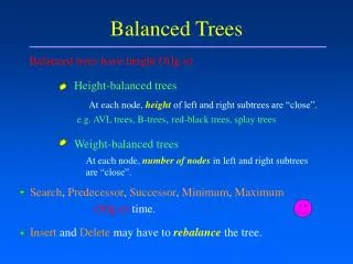
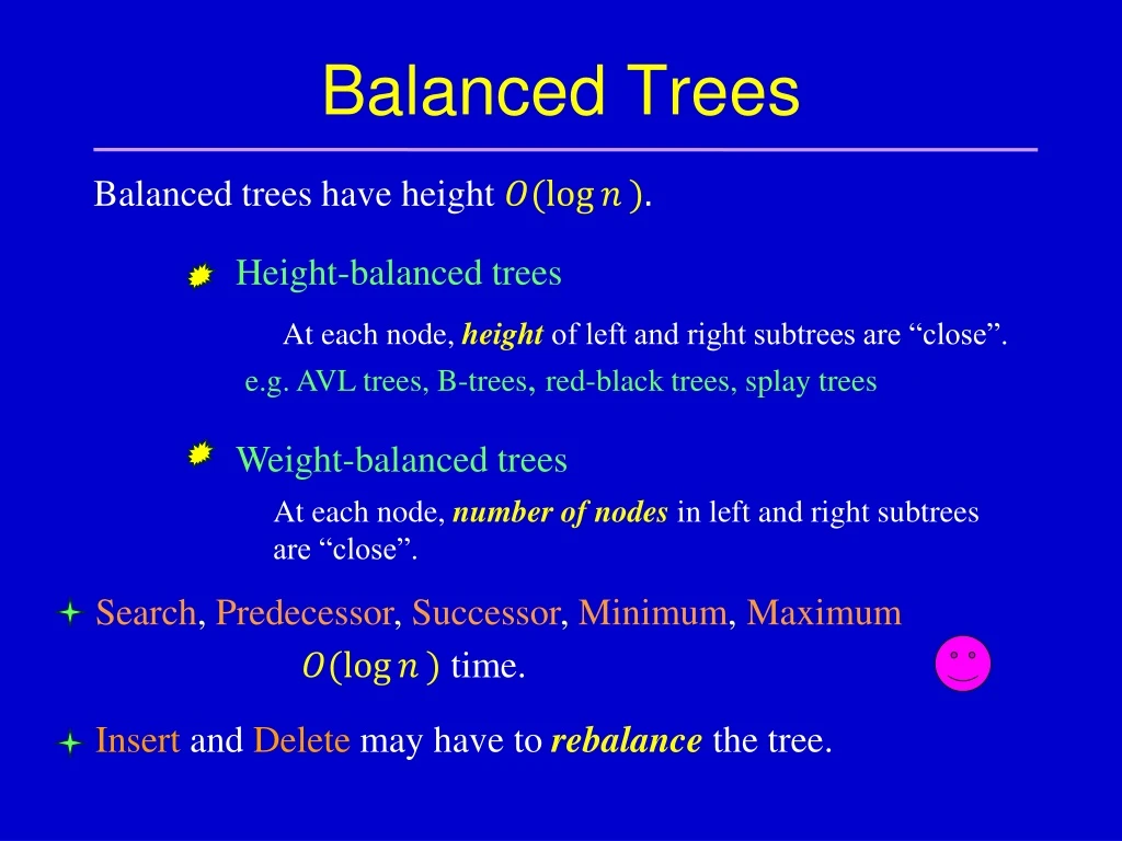
1. Height-balanced trees Weight-balanced trees Search, Predecessor, Successor, Minimum, Maximum Insert and Delete may have torebalancethe tree. Balanced Trees Balanced trees have height At each node,heightof left and right subtrees are “close”. e.g. AVL trees, B-trees,red-black trees, splay trees At each node,number of nodesin left and right subtrees are “close”. time.

2. Splay Trees Self-adjusting binary search tree (Sleator & Tarjan 1985) Amortized running time: Recently accessed elements are quick to access again. Averaged running time per operation over a worst-case sequence of operations.

3. Advantages Simple implementation –– easier to implement than other self-balancing BSTs such as red-black trees and AVL trees. Comparable performance –– average-case performance is as efficient as other self-balancing BSTs. Small memory footprint –– no need to store bookkeeping data. Working well with nodes containing identical keys.

4. Splaying Restructuring heuristics: Performs rotations bottom-up along the access path and moves the accessed item all the way to the root. Does the rotations in pairs, in an order depending on the structure of the access path. How to splaying a tree at a node ? Repeat a sequence of splaying steps until is the root of tree. zig, zig-zig, or zig-zag.

5. Case 1: zig Parent of is the tree root. Rotate the edge . rotate right Terminal case.

6. Case 1: zig (cont’d) rotate left

7. Case 2: zig-zig a) Parent of is not the root ( has grandparent ). b) and are both left or both right children. Symmetric rotations when and are both right children. Rotate Rotate

8. Case 3: zig-zag a) Parent of is not the root ( has grandparent ). b) is a left child and is a right child, or vice versa. Symmetric rotations when is a leftchild and is a rightchild. Rotate Rotate .

9. Time for Splaying a Node : where is the depth of the node . Proportional to the time to access the item stored in . Moves to the root. Roughly halves the depth of every node along the access path (shown in the next two examples). Effects of splaying:

10. Example 1 – Splay Step 1 J J Zig-zig Rotation 1 Splay Rotation 2 After rotation 1

11. Splay Step 2 J J Zig-zag Rotation 1

12. Splay Step 3 J J Zig-zag

13. Splay Step 4 J Zig-zig J E

14. Example 2 – All zig-zig Steps Splay

15. Example 2 (cont’d) Splay

16. Example 2 (cont’d) Splay

17. Example 3 – All zig-zag Steps

18. Example 3 (cont’d)

19. Example 3 (cont’d)

20. Data Access All BST update operations can be implemented by splaying. Access: if the item is stored in node , splay at ; otherwise, splay at the last non-null node (i.e., the leaf node) on the search path. Find 80: 70 50 50 90 Splay at 70 60 30 100 30 60 90 10 40 40 10 70 100 20 20 last non-null node 15 15

21. Insertion 1. Search for the item. 2. Create a new node containing the item if not in the tree. 3. Splay the tree at the new node. BST insertion + Splaying. Insert 80: 80 50 60 90 30 60 50 70 100 40 10 90 30 20 70 100 40 10 15 80 20 15

22. Joining Two BSTs Two BSTs and such that all items in are less than those in. Combine and into a single tree. is at the root. has no right child. Access the largest item in . It is stored in node . After the access: 2. Making the right subtree of this root.

23. Example 4 (of Join) : 50 : 30 60 40 10 90 120 120 20 70 100 15 110 110 140 140 100 100 50 50 90 90 30 30 40 40 60 60 10 10 20 20 70 70 15 15

24. Deletion 1. Search for the item (stored at with parent ). 2. Replace by the join of the left and right subtrees of . 3. Splay at (or the last node on the search path if the item is not found). Example Delete 30: 80 80 Join children of 30 60 60 90 90 50 50 70 100 70 100 20 30 40 40 10 10 20 15 15

25. Example 5 (cont’d) 50 80 Splay at 50 20 60 60 90 10 50 40 80 70 100 70 20 15 90 40 10 100 15 For more on splay trees, we refer to the following paper (where all examples but the joint one are from). D. D. Sleator and R. E. Tarjan. Self-adjusting binary search trees. Journal of the ACM, 32(3):652-686, 1985.