Translational diffusion: a sphere has the following frictional coefficient: f trans = 6πηR s .

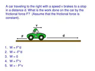
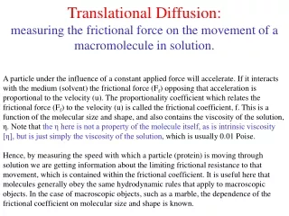
1. Translational Diffusion:measuring the frictional force on the movement of a macromolecule in solution. A particle under the influence of a constant applied force will accelerate. If it interacts with the medium (solvent) the frictional force (Ff) opposing that acceleration is proportional to the velocity (u). The proportionality coefficient which relates the frictional force (Ff) to the velocity (u) is called the frictional coefficient, f. This is a function of the molecular size and shape, and also contains the viscosity of the solution, η. Note that the η here is not a property of the molecule itself, as is intrinsic viscosity [η], but is just simply the viscosity of the solution, which is usually 0.01 Poise. Hence, by measuring the speed with which a particle (protein) is moving through solution we are getting information about the limiting frictional resistance to that movement, which is contained within the frictional coefficient. It is useful here that molecules generally obey the same hydrodynamic rules that apply to macroscopic objects. In the case of macroscopic objects, such as a marble, the dependence of the frictional coefficient on molecular size and shape is known.

2. Translational diffusion: a sphere has the following frictional coefficient: ftrans = 6πηRs. The larger the radius of a sphere, the larger the frictional coefficient, and the slower will be the velocity under a given driving force. Rotational diffusion: for a particle rotating in solution, there is also frictional resistance due to the shear force with the solvent. The hydrodynamics of this for a sphere is frot = 8πηRs3. Note that for rotational diffusion, the frictional coefficient increases in proportion to the volume of the sphere, whereas for translational diffusion, the dependence is proportional to the radius.

3. Diffusion Frictional Resistance to Macromolecule Motion Frictional Force (Ff) applied Force (Fap)  velocity, u Ff = f • u f  frictional coefficient steady state - terminal velocity is reached u = (Fap / f) For a sphere: ftrans = 6RS translational motion frot = 8RS3 rotational motion Measure molecular motion fRs molecular size and shape information

4. Diffusion is a purely statistical (or entropic) concept. It represents the net flow of matter from a region of high chemical potential (or concentration) to a region of low chemical potential. Diffusion can be considered as 1) the net displacement of a molecule after a large number of small random steps: random walk model. Alternatively, 2) it can also be looked at in terms of the net flow of matter under the influence of a gradient in the chemical potential, which can be formally treated as a hypothetical "force" field. Both approaches provide useful physical insight into how the diffusion of macromolecules can be utilized to yield molecular information. We will derive the concepts in terms of 1-dimension, and then generalize to 3-dimensions.

5. Translational diffusion • Phenomenological Equations Measured classically by observing the rate of “spreading” of the material: flux across a boundary Two equations relate the rate of change of concentration of particles as a function of position and time: Fick’s first law Fick’s second law

6. Flux of particles depends on the concentration gradient Fick’s first law Fick’s 1st law: J = -D moles (net) area • time dn dx J = flux  A  area of reference plane l l n1 n2 (concentration) Define the diffusion coefficient: D (cm2/sec)

7. dn (J1 - J2) A dt dx A = Change in concentration requires a difference in concentration gradient Fick’s second law area  A Fick’s 2nd law: = D change in # particles per unit time dn dt d2n dx2 volume dx J1 J2 Constant gradient: same amount leaves as enters the box Gradient higher on left: more enters the box than leaves

8. N 2 -x2 / 4 D t c(x,t) = ( D t)1/2 • e  solution Translational Diffusion Solve Fick’s Laws - differential equations ( relate concentration, position, time) (define boundary and initial conditions) diffusion in1 - dimension All (N) particles are at x = 0 at t = 0 Material spreads -5 -4 -3 -2 -1 0 1 2 3 4 5 (Gaussian) Note: <x2> = average value of x2 <x2> = p(x) dx • (x2) where p(x) is the probability of the molecules being at position x <x2> = 2 D t mean square displacement + -

9. Mean square displacement - in 3-dimensions isotropic diffusion Dx = Dy = Dz <x2> = 2Dt <y2> = 2Dt <z2> = 2Dt l2 = 6Dt where l2 = <x2> + <y2> + <z2> D = cm2/sec NOTE: Mean displacement   time l2 6t average displacement from the starting point = (6Dt)1/2

10. Values of Diffusion Coefficients 1. Diffusion in a gas phase: D  1 cm2/sec (will depend on length of λ , the mean free path) 2. Diffusion within a solid matrix: D ≈ 10-8 - 10-10 cm2/sec or much smaller 3. Diffusion of a small molecule in solution, such as sucrose in water at 25° C: D ≈ 10-5 cm2/sec (takes 3 days to go ~ 4 cm) 4. Diffusion of a macromolecule in solution, such as serum albumin (BSA, 70,000 mol weight) in water at 20° C: D ≈ 6 · 10-7 cm2/sec D  10-6 - 10-7 cm2/sec (3 days  1 cm) 5. Very large molecules such as DNA diffuse so slowly that the measurements cannot even be made. NOT a useful technique

11. Measuring the translational diffusion constant The classical method of measuring the translational diffusion constant is to observe the broadening of a boundary that is initially prepared by layering the protein solution on a solution without protein. In practice, this is not done. The preferred method for a purified protein is to use dynamic or quasi-elastic light scattering to get a value of the diffusion coefficient. The method measures the fluctuations in local concentrations of the protein within solution, and this depends on how fast the protein is randomly diffusing in the solution. There are commercial instruments to perform this measurement. Note that this does not yield a molecular weight but rather a Stokes radius. However, it is more common to use mass transport techniques to measure the Stokes radius of macromolecules. As we saw with osmotic pressure and with intrinsic viscosity, it is often necessary to make a series of diffusion measurements at different concentrations of protein and then extrapolate to infinite dilution. When this is done a superscript “0” is added: Do. The next slide shows results obtained for serum albumin.

12. Translational Diffusion Classical technique  boundary spread (mg/mL) start end x (distance) BSA Do 3.22 3.28 3.24 Extrapolate to infinite dilution (designated by Do) 107 x D * values of D have NOT been corrected for pure water at 20oC 0 5 10 15 C (mg/mL)

13. Another way to measure the value of the Diffusion Coefficient is by Fluorescence Correlation Spectroscopy (FCS) By measuring fluctuations in fluorescence, the residence time of a fluorescent molecule within a very small measuring volume (1 femtoliter, 10-15 L) is determined. This is related to the Diffusion Coefficient excitation emitted photons molecules moving into and out of the measuring volume: fast (left) vs slow (right) http://www.probes.com/handbook/boxes/1571.html

14. Fluorescence Correlation Spectroscopy: FCS the time-dependence of the fluorescence is expressed as an autocorrelation function, G(), the is the average value of the product of the fluorescence intensity at time t versus the intensity at a short time, , later. If the values fluctuate faster than time  then the product will be zero. deviation from the average intensity

15. An example of FCS: simulated autocorrelation functions of a free fluorescence ligand and the same ligand bound to a protein 1:1 mix of free/bound ligand bound ligand on slow moving protein G() goes to zero at long times free ligand (small, fast diffusion)

16. Relating D to molecular properties Rate of mass flux is inversely proportional to the frictional drag on the diffusing particle kT f k = Boltzman constant f = frictional coefficient D = But f = 6RS for a sphere or radius Rs  = viscosity of solution This expression appears to be valid for large objects such as marbles, and for macromolecules, and even for small molecules, at least to the extent that D·η is a constant for a molecule of fixed radius as the viscosity is changed. Stokes-Einstein Equation kT 6RS D =

17. Stokes Radius obtained from Diffusion kT Assumes a spherical shape 6RSStokes Radius kT 6D 1 You need additional information to judge whether the particle is really spherical -A highly asymmetric particle behaves like a larger sphere - higher frictional coefficient (f) 2 Deviations from the assumption of an anhydrous sphere (Rmin) are due to either a) hydration b) asymmetry 3 Stokes radius from different techniques need not be identical D = 2. Calculate Rs RS = 1. Measure D

18. Interpreting the meaning of the Stokes Radius b a kT kT f 6RS f = 6Rs Define: fmin = 6Rmin so: Rs f Rmin fmin Hydrodynamic theory defines the shape dependence of f, frictional coefficient D = = 1. Measure D and get Rs 2. Compare Rs to Rmin M N vol = [V2 • ] Rmin Experimental: 4 3 = R3min Theoretical: = this allows one to estimate effects due to molecular asymmetry (a / b) f / fmin

19. Shape factor for translational diffusion for a prolate ellipsoid frictional coefficient of ellipsoids oblate prolate f/fmin much larger effect of shape on viscosity than on diffusion viscosity shape factor frictional coefficient shape factor (Cantor + Schimmel)

20. Interpreting Diffusion Experiments:does a reasonable amount of hydration explain the measured value of D? Protein M Do20,W x10-7 cm2/s RS(Å) (diffusion) RNAse 13,683 11.9 18 (Rmin=17Å) Collagen 345,000 0.695 310 (Rmin=59Å) protein Maximum solvationMaximum asymmetry RNAse H2O = 0.35a/b = 3.4 Collagen H2O = 218a/b = 300 RS (Vp + H2O) 1/3 Rmin Vp solve for H2O Volume per gram of anhydrous protein =

21. What is the Diffusion Coefficient of a Protein in the bacterial cytoplasm? Are proteins freely mobile? Some proteins will be tethered Some proteins will interact transiently with others and appear to move slowly Free diffusion will be slower due to “crowding” effect excluded volume effect at high concentration of protein

22. Measuring the Diffusion of Proteins in the Cytoplasm of E. coli Fluorescence Recovery After Photobleaching (FRAP) Ready.. Aim... Fire! Diffusion of protein into the spot t1 t0 t2 E. coli cell 1. Express a protein that is fluorescent: green fluorescent protein, GFP. 2. Use a laser to “photo-bleach” the fluorescent protein in part of a single bacterial cell. This permanently destroys the fluorescence from proteins in the target area. 3. Measure the intensity of fluorescence as the protein diffuses into the region which was photo-bleached.

23. Diffusion of the Green Fluorescent Protein inside E. coli Single cell, expressing GFP Bleach cell center with a laser, t0 t = 0.37 sec after flash t = 1.8 sec after flash one can observe the molecules diffusing back into the bleached area 4 µm J. Bacteriology (1999) 181, 197-203

24. Diffusion of the Green Fluorescent Protein inside E. coli Results: D = 7.7 µm2/sec (7.7 x 10-8 cm2/sec) this is 11-fold less than the diffusion coefficient in water = 87 µm2/sec Slow translational diffusion is due to the crowding resulting from the very high protein concentration in the bacterial cytoplasm (200 -300 mg/ml) J. Bacteriology (1999) 181, 197-203