Download
1 / 101
1.01k likes | 1.03k Views
This presentation discusses the augmentation of the Nearest Neighbor Classifier to include a "don't know" option and explores different distance measures and feature generation techniques. It also introduces decision trees and the Naïve Bayes Classifier.

E N D
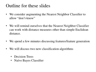
Outline for these slides • We consider augmenting the Nearest Neighbor Classifier to allow “don’t-know” • We will remind ourselves that the Nearest Neighbor Classifier can work with distance measures other than simple Euclidean distance. • We spend a few minutes discussing features/feature generation • We will discuss two new classification algorithms • Decision Trees • Naïve Bayes Classifier
Nearest Neighbor Classifier 10 9 8 7 6 5 4 3 2 1 1 2 3 4 5 6 7 8 9 10 Katydids Grasshoppers review Evelyn Fix 1904-1965 Joe Hodges 1922-2000 Antenna Length If the nearest instance to the previously unseen instance is a Katydid class is Katydid else class is Grasshopper Abdomen Length
Suppose we try to classy this insect. Its abdomen length suggests that it is as big as a cow! (it is clearly a typo). • What will the algorithm do? • What should the algorithm do? • The algorithm should say “dont-know” • We could achieve that a few ways. Suppose on our training set we measure N, the average distance of an object to its nearest neighbor (I did this, it was N = 2.7). • When we classify the new object, we could say either: • Nearest neighbor is red class: Warning: distance to nearest neighbor is 47 times the average distance, this is a low confidence result. • dont-know (because nearest_neighbor_dist > 3 * N) • Unlike professors, algorithms should say when they don’t know.
Minor point Sometimes the data type can be subjective, or depend on our interpretation. For example: I would say that eye colors are nominal, there are only 6 possibilities (Amber, Blue, Brown, Gray, Green, Hazel). But more generally, colors are interval data. Likewise, English letters are ordinal to us, we have A < B, and S < X etc. However a Japanese person with little exposure to the west might see the letters as being distinct and discrete, and therefore nominal, without realizing that they had any ordering.
10 9 8 7 6 5 4 3 2 1 1 2 3 4 5 6 7 8 9 10 Up to now we have assumed that the nearest neighbor algorithm uses the Euclidean Distance, however this need not be the case… Max (p=inf) Manhattan (p=1) Weighted Euclidean Mahalanobis
So far we have only seen features that are real numbers. But features could be: • Boolean (Has Wings?) • Nominal (Green, Brown, Gray) • etc How do we handle such features? The good news is that we can always define some measure of “nearest” for nearest neighbor for basically any kinds of features. Such measures are called distance measures (or sometime, similarity measures).
Let us consider an example that uses Boolean features: • Features: • Has wings? • Has spur on front legs? • Has cone-shaped head? • length(antenna) > 1.5* length(abdomen) (real values converted to Boolean) • Under this representation, every insect is a just Boolean vector: • Insect17 ={true, true, false, false} • or • Insect17 ={1,1,0,0} • Instead of using the Euclidean distance, we can use the Hamming distance (or one of many other measures). • Which insect is the nearest neighbor of Insect17 ={1,1,0,0}? • Insect1 ={1,1,0,1}, Insect2 ={0,0,0,0}, Insect3 ={0,1,1,1}, Insect3 ={0,1,1,1} • Here we would say Insect17 is in the blue class. Insect17 The Hamming distance between two strings of equal length is the number of positions at which the corresponding symbols are different.
We have seen a distance measures for real-valued data (Euclidean distance). We have seen a distance measures for Ordinal data (string-edit distance). We have seen a distance measure for Nominal (Boolean) data (Hamming distance). In coming week, we will see that there many distance measures, for all kinds of data, and even mixtures of data types.
For any domain of interest, we can measure features Color {Green, Brown, Gray, Other} Has Wings? Abdomen Length Thorax Length Antennae Length Mandible Size Spiracle Diameter Leg Length
5 2.5 10 9 8 7 6 2 5 5 4 3 2 1 5 3 1 2 3 4 5 6 7 8 10 9 2.5 3 Feature Generation • Feature generation refers to any technique to make new features from existing features • Recall pigeon problem 2, and assume we are using the linear classifier Pigeon Problem 2 Examples of class A Examples of class B Using both features works poorly, using just X works poorly, using just Y works poorly.. 4 4 5 5 6 6 3 3
10 9 8 7 6 5 4 3 2 1 1 2 3 4 5 6 7 8 10 9 Feature Generation • Solution: Create a new feature Z Z = absolute_value(X-Y) 0 1 2 3 4 5 6 7 8 10 9 Z-axis
Recall this example? It was a teaching example to show that NN could use any distance measure It would not really work very well, unless we had LOTS more data…
What features can we use classify Japanese names vs Irish names? • The first letter = ‘A’ ? (Boolean feature) Useless Japanese Names Irish Names ABERCROMBIE ABERNETHY ACKART ACKERMAN ACKERS ACKLAND ACTON ADAIR ADLAM ADOLPH AFFLECK AIKO AIMI AINA AIRI AKANE AKEMI AKI AKIKO AKIO AKIRA AMI AOI ARATA ASUKA
What features can we use classify Japanese names vs Irish names? • The first letter = ‘A’ ? (Boolean feature) Useless • The first letter of name (Nominal or Ordinal feature) Useless (but not useless for Chinese vs Irish, there are very few Irish names that begin with ‘X’, ‘Z’, ‘W’) Japanese Names Irish Names ABERCROMBIE ABERNETHY ACKART ACKERMAN ACKERS ACKLAND ACTON ADAIR ADLAM ADOLPH AFFLECK AIKO AIMI AINA AIRI AKANE AKEMI AKI AKIKO AKIO AKIRA AMI AOI ARATA ASUKA
What features can we use classify Japanese names vs Irish names? • The first letter = ‘A’ ? (Boolean feature) Useless • The first letter of name (Nominal or Ordinal feature) Useless (but not useless for Chinese vs Irish, there are few Irish names that begin with ‘X’, ‘Z’, ‘W’) • The number of letters in the name (Ratio feature) Slightly useful, Irish names are a litter longer on average. Japanese Names Irish Names ABERCROMBIE ABERNETHY ACKART ACKERMAN ACKERS ACKLAND ACTON ADAIR ADLAM ADOLPH AFFLECK AIKO AIMI AINA AIRI AKANE AKEMI AKI AKIKO AKIO AKIRA AMI AOI ARATA ASUKA
What features can we use classify Japanese names vs Irish names? • The first letter = ‘A’ ? (Boolean feature) Useless • The first letter of name (Nominal or Ordinal feature) Useless (but not useless for Chinese vs Irish, there are few Irish names that begin with ‘X’, ‘Z’, ‘W’) • The number of letters in the name (Ratio feature) Slightly useful, Irish names are a litter longer on average. • The last letter of name (Nominal or Ordinal feature) Somewhat useful, more Japanese names end in “I” (girls) or “O” (boys), than Irish names do. Japanese Names Irish Names ABERCROMBIE ABERNETHY ACKART ACKERMAN ACKERS ACKLAND ACTON ADAIR ADLAM ADOLPH AFFLECK AIKO AIMI AINA AIRI AKANE AKEMI AKI AKIKO AKIO AKIRA AMI AOI ARATA ASUKA
The number of vowels / world length (Ratio feature) Useful, Japanese names tend to have proportionally more vowels than Irish names. Japanese Names Irish Names ABERCROMBIE 0.45 ABERNETHY 0.33 ACKART 0.33 ACKERMAN 0.375 ACKERS 0.33 ACKLAND 0.28 ACTON 0.33 AIKO 0.75 AIMI 0.75 AINA 0.75 AIRI 0.75 AKANE 0.6 AKEMI 0.6 Vowels = I O U A E
This little example of feature generation is something data miners spend a lot of time doing. With the right features, most algorithms will work well. Without the right features, no algorithm will work well. There is no single trick that always works, but as we “play” with more and more datasets, we get better at feature generation over time. What feature(s) do we use here?
Classification We have seen 2 classification techniques: • Simple linear classifier, Nearest neighbor,. Let us see two more techniques: • Decision tree, Naïve Bayes There are other techniques: • Neural Networks, Support Vector Machines, … that we will not consider..
I have a box of apples.. 1 H(X) Pr(X = good) = p then Pr(X = bad) = 1 − p the entropy of X is given by 0.5 0 0 binary entropy function attains its maximum value when p = 0.5 1 All good All bad
Decision Tree Classifier 10 9 8 7 6 5 4 3 2 1 1 2 3 4 5 6 7 8 9 10 Ross Quinlan Abdomen Length > 7.1? Antenna Length yes no Antenna Length > 6.0? Katydid yes no Katydid Grasshopper Abdomen Length
Antennae shorter than body? Yes No 3 Tarsi? Grasshopper Yes No Foretiba has ears? Yes No Cricket Decision trees predate computers Katydids Camel Cricket
Decision Tree Classification • Decision tree • A flow-chart-like tree structure • Internal node denotes a test on an attribute • Branch represents an outcome of the test • Leaf nodes represent class labels or class distribution • Decision tree generation consists of two phases • Tree construction • At start, all the training examples are at the root • Partition examples recursively based on selected attributes • Tree pruning • Identify and remove branches that reflect noise or outliers • Use of decision tree: Classifying an unknown sample • Test the attribute values of the sample against the decision tree
How do we construct the decision tree? • Basic algorithm (a greedy algorithm) • Tree is constructed in a top-down recursive divide-and-conquer manner • At start, all the training examples are at the root • Attributes are categorical (if continuous-valued, they can be discretized in advance) • Examples are partitioned recursively based on selected attributes. • Test attributes are selected on the basis of a heuristic or statistical measure (e.g., information gain) • Conditions for stopping partitioning • All samples for a given node belong to the same class • There are no remaining attributes for further partitioning – majority voting is employed for classifying the leaf • There are no samples left
Information Gain as A Splitting Criteria • Select the attribute with the highest information gain (information gain is the expected reduction in entropy). • Assume there are two classes, P and N • Let the set of examples S contain p elements of class P and n elements of class N • The amount of information, needed to decide if an arbitrary example in S belongs to P or N is defined as 0 log(0) is defined as0
Information Gain in Decision Tree Induction • Assume that using attribute A, a current set will be partitioned into some number of child sets • The encoding information that would be gained by branching on A Note: entropy is at its minimum if the collection of objects is completely uniform
Entropy(4F,5M) = -(4/9)log2(4/9) - (5/9)log2(5/9) = 0.9911 no yes Hair Length <= 5? Let us try splitting on Hair length Entropy(3F,2M) = -(3/5)log2(3/5) - (2/5)log2(2/5) = 0.9710 Entropy(1F,3M) = -(1/4)log2(1/4) - (3/4)log2(3/4) = 0.8113 Gain(Hair Length <= 5) = 0.9911 – (4/9 * 0.8113 + 5/9 * 0.9710 ) = 0.0911
Entropy(4F,5M) = -(4/9)log2(4/9) - (5/9)log2(5/9) = 0.9911 no yes Weight <= 160? Let us try splitting on Weight Entropy(0F,4M) = -(0/4)log2(0/4) - (4/4)log2(4/4) = 0 Entropy(4F,1M) = -(4/5)log2(4/5) - (1/5)log2(1/5) = 0.7219 Gain(Weight <= 160) = 0.9911 – (5/9 * 0.7219 + 4/9 * 0 ) = 0.5900
Entropy(4F,5M) = -(4/9)log2(4/9) - (5/9)log2(5/9) = 0.9911 no yes age <= 40? Let us try splitting on Age Entropy(1F,2M) = -(1/3)log2(1/3) - (2/3)log2(2/3) = 0.9183 Entropy(3F,3M) = -(3/6)log2(3/6) - (3/6)log2(3/6) = 1 Gain(Age <= 40) = 0.9911 – (6/9 * 1 + 3/9 * 0.9183 ) = 0.0183
Of the 3 features we had, Weight was best. But while people who weigh over 160 are perfectly classified (as males), the under 160 people are not perfectly classified… So we simply recurse! no yes Weight <= 160? This time we find that we can split on Hair length, and we are done! no yes Hair Length <= 2?
We need don’t need to keep the data around, just the test conditions. Weight <= 160? yes no How would these people be classified? Hair Length <= 2? Male yes no Male Female
It is possible that when we are building a decision tree, we have a node that is not pure, but we have no more features to test (or the feature tests don’t suggest a split). What can we do? yes • We can report “don’t know”. Sometimes that would work. For example. If a decision tree is processing credit card applications, we give a credit to “Yes” but not to “No” or “Don’t know”. The might be a little lost opportunity there, but if “Don’t know” is rare, it will not matter. In some cases, we cannot do this. Every email has to be a spam or no-spam. Interesting example: For an ATM check-reader, if it can classify each number, then it registers that amount. If one of the numbers is classified as “Don’t know”, then the image is sent to a outsourced human.
It is possible that when we are building a decision tree, we have a node that is not pure, but we have no more features to test (or the feature tests don’t suggest a split). What can we do? yes • We can report “don’t know”. Sometimes that would work. For example. If a decision tree is processing credit card applications, we give a credit to “Yes” but not to “No” or “Don’t know”. The might be a little lost opportunity there, but if “Don’t know” is rare, it will not matter. In some cases, we cannot do this. Every email has to be a spam or no-spam. • We can report a probability. So, for example, if a new instance arrives at the node above, we would report: Male with 75% confidence.
It is trivial to convert Decision Trees to rules… Weight <= 160? yes no Hair Length <= 2? Male no yes Male Female Rules to Classify Males/Females IfWeightgreater than 160, classify as Male Elseif Hair Lengthless than or equal to 2, classify as Male Else classify as Female
Once we have learned the decision tree, we don’t even need a computer! This decision tree is attached to a medical machine, and is designed to help nurses make decisions about what type of doctor to call. Decision tree for a typical shared-care setting applying the system for the diagnosis of prostatic obstructions.
PSA = serum prostate-specific antigen levels PSAD = PSA density TRUS = transrectal ultrasound Garzotto M et al. JCO 2005;23:4322-4329
Classification Problem: Fourth Amendment Cases before the Supreme Court II The Supreme Court’s search and seizure decisions, 1962–1984 terms. Keogh vs. State of California = {0,1,1,0,0,0,1,0} U = Unreasonable R = Reasonable
We can also learn decision trees for individual Supreme Court Members. Using similar decision trees for the other eight justices, these models correctly predicted the majority opinion in 75 percent of the cases, substantially outperforming the experts' 59 percent. Decision Tree for Supreme Court Justice Sandra Day O'Connor
The worked examples we have seen were performed on small datasets. However with small datasets there is a great danger of overfitting the data… When you have few datapoints, there are many possible splitting rules that perfectly classify the data, but will not generalize to future datasets. Yes No Wears green? Male Female For example, the rule “Wears green?” perfectly classifies the data, so does “Mothers name is Jacqueline?”, so does “Has blue shoes”…
Avoid Overfitting in Classification • The generated tree may overfit the training data • Too many branches, some may reflect anomalies due to noise or outliers • Result is in poor accuracy for unseen samples • Two approaches to avoid overfitting • Prepruning: Halt tree construction early—do not split a node if this would result in the goodness measure falling below a threshold • Difficult to choose an appropriate threshold • Postpruning: Remove branches from a “fully grown” tree—get a sequence of progressively pruned trees • Use a set of data different from the training data to decide which is the “best pruned tree”
10 10 100 9 9 90 8 8 80 7 7 70 6 6 60 5 5 50 4 4 40 3 3 30 2 2 20 1 1 10 1 1 2 2 3 3 4 4 5 5 6 6 7 7 8 8 10 10 9 9 10 20 30 40 50 60 70 80 100 90 Which of the “Pigeon Problems” can be solved by a Decision Tree? • Deep Bushy Tree • Useless • Deep Bushy Tree ? The Decision Tree has a hard time with correlated attributes
Advantages/Disadvantages of Decision Trees • Advantages: • Easy to understand (Doctors love them!) • Easy to generate rules • Disadvantages: • May suffer from overfitting. • Classifies by rectangular partitioning (so does not handle correlated features very well). • Can be quite large – pruning is necessary. • Does not handle streaming data easily
How would we go about building a classifier for projectile points? ?
length I. Location of maximum blade width 1. Proximal quarter 2. Secondmost proximal quarter 3. Secondmost distal quarter 4. Distal quarter II. Base shape 1. Arc-shaped 2. Normal curve 3. Triangular 4. Folsomoid III. Basal indentation ratio 1. No basal indentation 2. 0·90–0·99 (shallow) 3. 0·80–0·89 (deep) IV. Constriction ratio • 1·00 • 0·90–0·99 • 0·80–0·89 4. 0·70–0·79 5. 0·60–0·69 • 0·50–0·59 V. Outer tang angle 1. 93–115 2. 88–92 3. 81–87 4. 66–88 5. 51–65 6. <50 VI. Tang-tip shape 1. Pointed 2. Round 3. Blunt VII. Fluting 1. Absent 2. Present VIII. Length/width ratio 1. 1·00–1·99 2.2·00–2·99 3. 3.00 -3.99 4. 4·00–4·99 5. 5·00–5·99 6. >6. 6·00 width 21225212 length = 3.10 width = 1.45 length /width ratio= 2.13
I. Location of maximum blade width 1. Proximal quarter 2. Secondmost proximal quarter 3. Secondmost distal quarter 4. Distal quarter II. Base shape 1. Arc-shaped 2. Normal curve 3. Triangular 4. Folsomoid III. Basal indentation ratio 1. No basal indentation 2. 0·90–0·99 (shallow) 3. 0·80–0·89 (deep) IV. Constriction ratio • 1·00 • 0·90–0·99 • 0·80–0·89 4. 0·70–0·79 5. 0·60–0·69 • 0·50–0·59 V. Outer tang angle 1. 93–115 2. 88–92 3. 81–87 4. 66–88 5. 51–65 6. <50 VI. Tang-tip shape 1. Pointed 2. Round 3. Blunt VII. Fluting 1. Absent 2. Present VIII. Length/width ratio 1. 1·00–1·99 2.2·00–2·99 3. 3.00 -3.99 4. 4·00–4·99 5. 5·00–5·99 6. >6. 6·00 21225212 Fluting? = TRUE? yes no Base Shape = 4 Late Archaic yes no Length/width ratio = 2 Mississippian
We could also us the Nearest Neighbor Algorithm ? 21225212 21265122 - Late Archaic 14114214 - Transitional Paleo 24225124 - Transitional Paleo 41161212 - Late Archaic 33222214 - Woodland
Avonlea Clovis 1.5 1.0 0.5 11.24 I (Clovis) 0 85.47 II (Avonlea) Shapelet Dictionary 0 100 200 300 400 Arrowhead Decision Tree I II 0 2 1 Clovis Mix Avonlea Decision Tree for Arrowheads It might be better to use the shape directly in the decision tree… Lexiang Ye and Eamonn Keogh (2009) Time Series Shapelets: A New Primitive for Data Mining. SIGKDD 2009 Training data (subset) The shapelet decision tree classifier achieves an accuracy of 80.0%, the accuracy of rotation invariant one-nearest-neighbor classifier is 68.0%.
Decision Tree for Shields Training data (subset) The shapelet decision tree classifier achieves an accuracy of 89.9%, the accuracy of rotation invariant one-nearest-neighbor classifier is 82.9%.