Dealing with Exponential Problems

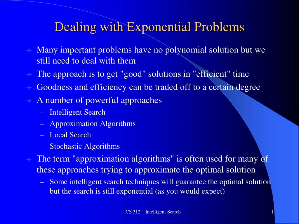
1. Dealing with Exponential Problems • Many important problems have no polynomial solution but we still need to deal with them • The approach is to get "good" solutions in "efficient" time • Goodness and efficiency can be traded off to a certain degree • A number of powerful approaches • Intelligent Search • Approximation Algorithms • Local Search • Stochastic Algorithms • The term "approximation algorithms" is often used for many of these approaches trying to approximate the optimal solution • Some intelligent search techniques will guarantee the optimal solution but the search is still exponential (as you would expect) CS 312 – Intelligent Search

2. Intelligent Search • The full problem is made up of an exponential search space and thus exhaustive search is exponential • Informed (intelligent) vs. uninformed search • Intelligent search seeks to reduce the number of states we actually search by one or both of the following: • Pruning, as soon as possible, branches of the search tree which cannot lead to a solution • Trying first those branches which are most promising in hopes of finding a reasonable solution quickly, thus avoiding alternatives • Approaches • Backtracking • Branch and Bound • Beam Search – Non optimal solution, but faster • A* search CS 312 – Intelligent Search

3. Backtracking • Natural for decision search problems • Is there a solution or not • SAT – Satisfiability • Does there exist a setting of Boolean variables which satisfies a particular CNF Boolean expression – 2n possible settings • NP-complete problem • Verifiable in polynomial time – Easy to test • What is simple algorithm/complexity? • What does full search tree look like? • Backtracking allows us to prune branches • Branch on arbitrary variable (e.g. w) • Both leafs still possible, but when we branch on x, note that the leaf (w=0, x=1) is impossible so we can prune all subtrees of that node – can backtrack out of that dead-end CS 312 – Intelligent Search

4. Backtracking with SAT • Clauses in a node represent what still remains to be satisfied • Dropping a clause in a node means that the clause is satisfied • If we find any empty node (i.e. all clauses satisfied) then full expression is satisfiable • An empty clause signifies that the clause is not satisfiable and we can prune that path • If all leafs contain an empty clause then the expression is not satisfiable

5. Backtracking Algorithm • Backtracking is still exponential, but due to the pruning it is more practical in many cases • More room to increase the size of the problem before it becomes intractable CS 312 – Intelligent Search

6. Branch and Bound • Similar to Backtracking but applied to optimization problems • Common and powerful technique for many tasks • For a minimization problem, we need an efficient/quick mechanism to generate an optimistic lowerbound(S) for a particular state S (or upperbound for maximization) • From S we know that we could never get a better solution than lowerbound(S) – Note we want LB(S) as big as possible • We keep track of the Best Solution So Far (BSSF) • If lowerbound(S) ≥ BSSF then we can prune S and not search anymore below it • The better (tighter) the bounding function the more we can prune the search CS 312 – Intelligent Search

7. Branch and Bound Algorithm • B&B returns the optimal solution • Just like backtracking, B&B is still exponential, but often runs in relatively fast time due to pruning and depending on the quality of the bounding function • Before expanding a problem PS, make sure its' LB is still < BSSF, since BSSF may have been updated since P was put in the set S • Also, as a heuristic, could make S a priority queue with LB(P) as the key – always expand P with lowest LB as a heuristic • All P with LB < BSSF must be expanded before we terminate, to be optimal CS 312 – Intelligent Search

8. Bounding Function Example – 15 puzzle • Want the least number of moves necessary to complete the puzzle • What does the search space look like? • What kind of bounding function could we use to help prune space? • Must never over-estimate the actual optimum (is a lower-bound) • Can we do better? • The closer the bound can get to the actual optimum, the more we can prune • The bounding function should be relatively fast to compute • Would if bound estimate overestimated needed steps from the state? CS 312 – Intelligent Search

9. Beam Search • A beam search is a semi-greedy state space search that only keeps a limited specified number (the beam width) of states in memory • When the state space exceeds the beam width, then all the states with the worst bound/heuristic value are dropped • Thus it is sub-optimal since the optimal solution may have been in one of the dropped states • More efficient in both time and space • Memory is controlled explicitly by the beam width • Can make B&B a beam search by putting a max (beam width) on the number of states to save. Common approach. CS 312 – Intelligent Search

10. TSP B&B: State Space • The complete solutions are the (n-1)! leaves • One for each possible path • Would like an efficient bounding function for each state which could allow pruning to avoid searching all states • What is the loosest and what is the tightest bound? • What are some other bounds? CS 312 – Intelligent Search

11. TSP B&B: State Space • Would like an efficient bounding function for each state which could allow pruning to avoid searching all states • Current partial distance + sum of the shortest edges leaving remaining nodes • Current partial distance + MST(remaining nodes) • etc. • Note that we also need a search space strategy that drills down to some final states so we can keep updating BSSF to allow better pruning CS 312 – Intelligent Search

12. Reduced Cost Matrix Approach As long as the bound is optimistic (≤ the optimal tour), branch and bound will return the optimal path for TSP You will implement this bounding approach for your project, together with an improved state space search We will not give you exact pseudo-code for this project, but will review approaches in the slides and make available some pertinent reading material n city problem – Directed graph version – can have asymmetric city distances TSP is a Hamiltonian Cycle, also called a Rudrata Cycle CS 312 – Intelligent Search

13. 1 2 5 3 4 Bound on TSP Tour 9 1 8 2 10 6 4 3 12 7 4 Hint: Every tour must leave every vertex and arrive at every vertex. Any proposals?

14. Bound on TSP Tour • Could use sum of smallest exiting edge from each vertex • or similarly, Could use sum of smallest entering edge into each vertex • Are these optimistic? • Can do even better if we can combine both • Sum them? • Do one first, then somehow sum in the residual of the other, given the first CS 312 – Intelligent Search

15. 1 2 5 3 4 Bound on TSP Tour 9 1 8 2 10 6 4 3 12 7 4 What’s the cheapest way to leave each vertex? CS 312 – Intelligent Search

16. 1 2 5 3 4 Bound on TSP Tour Initial rough bound= 8+2+3+6+1 = 20 9 1 8 2 6 10 4 3 12 7 4 Save the sum of those costs in the bound (as a first draft). Still can gain better bound by making sure we arrive at each vertex CS 312 – Intelligent Search

17. 1 2 5 3 4 Reduced Cost Matrix Rough draft bound = 20 9-8=1 1 8-8=0 2 10 6 4 3 12 7 4 For a given vertex, subtract the least departure edge cost from each edge leaving that vertex. This leaves the potential increased cost of taking a different edge in the reduced cost matrix. If we decide later to use edge (1,2) instead of (1,4), the cost would be only 1 more (9) than we already had (8).

18. 1 2 5 3 4 Reduced Cost Matrix Rough draft bound = 20 1 0 0 0 9 0 2 0 6 1 1 Repeat for the other vertices. Now, let's find a tighter lower bound. Does the set of edges now having 0 residual cost (those making up our current bound) arrive at every vertex? – No. None into vertex 3

19. 1 2 5 3 4 Bound on TSP Tour Rough draft bound = 20 1 0 0 0 9 0 2 0 6 1 1 We have to take an edge to vertex 3 from somewhere. Assume we take the cheapest currently available.

20. 1 2 5 3 4 Bound on TSP Tour Bound = 21 1 0 0 0 9 0 1 0 6 0 1 Subtract this cheapest edge cost from all edges entering vertex 3 and add the cost to the bound. We do this for all vertices which did not have an in-bound edge of 0 cost to complete our reduced cost matrix. We have just tightened the bound.

21. The Bound • It will cost at least this much to visit all the vertices in the graph. • There is no cheaper way to get in and out of each vertex. • The edges in our reduced cost matrix are now labeled with the extra cost of choosing that edge. • Remember, the bound is not necessarily (and not usually) a solution, and for minimization is always ≤ optimal solution CS 312 – Intelligent Search

22. 9 1 1 8 2 2 5 10 6 4 3 12 7 3 4 4 Cost Matrix We can accomplish the steps of this algorithm using a cost matrix CS 312 – Intelligent Search

23. 1 0 1 0 0 2 5 9 0 2 0 6 1 3 4 1 Reduced Cost Matrix Reduce all rows by subtracting the minimum path from the other path lengths. Sum the reduction amounts as we go to build the bound. Initial rough bound= 8+2+3+6+1 = 20

24. 1 0 1 0 0 2 5 9 0 2 0 6 1 3 4 1 Reduced Cost Matrix Then reduce all columns by subtracting the minimum path lengths and adding them to the bound. Only column 3 reduces since it has no 0's. Now we have a tighter bound. Note that there is now at least one 0 in every row and column. final bound = 20 + 1 = 21

25. Reduced Cost Matrix Algorithm bound = 0 initially (or is the bound of the parent state) For each row in A Subtract the minimum cell value in the row from all cells in the row and add that value to the bound Then for each column in A Subtract the minimum cell value in the column from all cells in the column and add that value to the bound At that point every column and row will have at least one 0 entry and we will have the correct bound summed

26. Reduced Cost Matrix Algorithm • Could have done columns first and then rows • Which is better? • Still give a correct lower bound, but not necessarily the same reduced cost matrix as the row first approach • Could try both, but then we have the trade-off of more time vs finding a better bound CS 312 – Intelligent Search

27. 1 2 5 3 4 Initial BSSF Initial BSSF Value: Infinite? A tighter value would lead to more initial pruning. Should be quick to calculate, but best if it is a reasonable value, since it may take a while before your first complete solutions finish and allow BSSF update Don't use reduced matrix value because it will be lower than the optimal and algorithm would not be complete. BSSF is opposite of the bound in that it must be ≥ the optimal path (upper bound) - Want BSSF as small as possible Could try a few random legal paths and pick the best. Be creative on this for your project. Can make a significant difference. 9 1 8 2 10 6 5 3 12 7 4

28. 1 2 5 3 4 Random BSSF Cost of random BSSF = 9+5+4+12+1 = 31 Want BSSF as low as possible andLB as high as possible Where does optimal lie? 9 1 8 2 10 6 5 3 12 7 4 CS 312 – Intelligent Search

29. State Space Search • The state space search approach defines the manner in which children (or “successor”) states are expanded from a given state in the state space search (i.e. How we search through the tree). This is the search "frontier," which in this case is stored in the priority queue. • We will introduce two approaches • The first assumes each state represents a partial path • A link to a child state represents a path from the root city to the child • We will arbitrarily make the first state represent city 1 • Children states in the search tree are generated by considering each path leaving the parent city in the TSP graph. We then calculate the reduced cost matrix for each child state and put child states whose bound is less than the BSSF on a priority queue where the bound is the PQ key • Do we need to use a priority queue? • Note that the initial reduced cost matrix is the same regardless of which node we started at CS 312 – Intelligent Search

30. Partial Path State Space CS 312 – Intelligent Search

31. 1 2 5 4 3 State Space Search – Partial Path State 1 (21) BSSF = 31 Don't confuse search state number with city number 9 1 8 2 (1,3) (1,2) (1,4) (1,5) 6 10 State 2 State 4 State 5 State 3 4 3 7 What changes? bound = 21 + ? 12 4 S6 S7 S8 S9 S10 S11 S12 S13 S14 S15 S16 S17

32. 1 2 5 4 3 State Space Search – Partial Path State 1 (21) BSSF = 31 Don't confuse search state number with city number 9 1 8 2 (1,3) (1,2) (1,4) (1,5) 6 10 State 2 State 4 State 5 State 3 4 3 7 • What changes? (row:fromcolumn:to) • bound = 21 + 1 (cost of edge) + ? • First set "from row" and "to column" = ∞ • also for selected edge (i,j), set (j,i) = ∞ 12 4 S6 S7 S8 S9 S10 S11 S12 S13 S14 S15 S16 S17

33. 1 2 5 4 3 State Space Search – Partial Path State 1 (21) BSSF = 31 Don't confuse search state number with city number 9 1 8 2 (1,3) (1,2) (1,4) (1,5) 6 10 State 2 State 4 State 5 State 3 4 3 7 What changes? (row:fromcolumn:to) bound = 21 + 1 + 1 = 23 = prev bound+ path(1,2) + cost of reducing the updated cost matrix 12 4 S6 S7 S8 S9 S10 S11 S12 S13 S14 S15 S16 S17

34. 1 2 5 4 3 State Space Search – Partial Path State 1 (21) BSSF = 31 Don't confuse search state number with city number 9 1 8 2 (1,3) (1,2) (1,4) (1,5) 6 10 State 2 (21+1+1=23) State 4 (21+0+0=21) State 5 (21+∞+∞=∞) State 3 (21+∞+1=∞) 4 3 7 12 4 S6 S7 S8 S9 S10 S11 S12 S13 S14 S15 S16 S17

35. State Space Search • To create each new state, start with the bound for the parent state and • Add the residual cost of the new path • Set to infinity paths which can no longer be used (row of from-state, column of to-state, and to,from state) • Reduce the new matrix and add the cost of reduction • States 3 and 5 will be pruned • States 2 and 4 will be enqueued and state 4 (with the lowest bound 21) will be the first on the queue and the next state expanded if using a priority queue • Adjust BSSF? - Not until we have a complete solution which is better • Number of remaining edges in the graph decrease at each level of the tree

36. 1 2 5 4 3 State Space Search State 4 (21) BSSF = 31 9 1 8 2 Went from city 1 to 4 6 10 4 3 7 12 4

37. 1 2 5 4 3 State Space Search State 4 (21) BSSF = 31 9 1 8 2 (4,3) (4,2) (4,5) 6 10 State 12 (21+0+∞=∞) State 14 (21+6+1)=28 State 13 (21+0+0=21) 4 3 7 12 13 and 14 will be put on the queue with State 13 the lowest 4

38. 1 2 5 4 3 State Space Search State 13 (21) Path so far 1, 4, 3 BSSF = 31 9 1 8 2 Just the first state is put in the queue and it will then select path 2-5 with no new added cost. The last step will be the path 5-1 which also has no added cost (3,2) (3,5) 6 10 (21+∞+0)=∞ (21+0+0=21) 4 3 7 12 4

39. Search Tree for Partial Path Search Complete path at bottom state is 1 – 4 – 3 – 2 – 5 – 1 Total Distance = 21 Once we hit the first complete solution, BSSF is updated to 21 In this case the two states on the queue (23, 28) will be pruned as soon as they are dequeued, leaving the queue empty and the algorithm will stop and return 21 If there had been states on the queue with a bound lower than the updated BSSF, then processing would have continued b=21 1-to-2 1-to-4 b=23 b=21 4-to-2 4-to-3 4-to-5 b=21 b=28 b=∞ 3-to-2 b=21 2-to-5 5-to-1 CS 312 – Intelligent Search

40. Partial Path B&B Complexity Number of node expansions required? CS 312 – Intelligent Search

41. Partial Path B&B Complexity • Number of node expansions required? O(bn) where b is the average state branching factor and n is the depth of solutions • Note it is not a balanced tree, but the frontier still grows exponentially • The hope is that pruning will keep the branching factor down and also keep the tree more shallow in many places • Space Complexity? CS 312 – Intelligent Search

42. Partial Path B&B Complexity • Number of node expansions required? O(bn) where b is the average state branching factor and n is the depth of solutions • Note it is not a balanced tree, but the frontier still grows exponentially • The hope is that pruning will keep the branching factor down and also keep the tree more shallow in many places • Space Complexity? O(n2bn) since we store one reduced cost matrix (n2) for each node in the queue and the queue is the frontier of the search tree which is O(bn) • Time Complexity? CS 312 – Intelligent Search

43. Partial Path B&B Complexity • Number of node expansions required? O(bn) where b is the average state branching factor and n is the depth of solutions • Note it is not a balanced tree, but the frontier still grows exponentially • The hope is that pruning will keep the branching factor down and also keep the tree more shallow in many places • Space Complexity? O(n2bn) since we store one reduced cost matrix (n2) for each node in the queue and the queue is the frontier of the search tree which is O(bn) • Time Complexity? – O(n2bn), the number of nodes created for potential queue insertion, times the complexity of creating a node which is the cost of reducing the cost matrix which is O(n2) CS 312 – Intelligent Search

44. Improved State Space Search • We used a priority queue so that the state with the best (lowest) bound can be chosen when it is time to expand a new state • For the partial path state space search this can lead to a fairly broad (breadth-first) search frontier • All O(n) child states are calculated (and many put in the queue) each time a state is expanded • Leads to a large number of states in the priority queue • Also, BSSF is not updated until a completed path node (leaf) is reached which could be a while for large n • Can we use a different state space to gain advantage? • We can still use the same bounding scheme – reduced cost matrix • Want a state space search that "drills deeper" leading to finding complete paths which will update the BSSF sooner and lead to earlier pruning CS 312 – Intelligent Search

45. Include/Exclude State Space Search • Include/Exclude approach improves TSP performance compared to the partial path approach and you will use it for your project • We'll use the same reduced cost matrix bounding function, though any bounding function could be used • We do not choose an initial city to start at; we just have the initial reduced cost matrix tied to the initial search state • The search tree will be a binary tree with the decision based on whether a particular edge is in the final solution or out of it Include edge (i,j) Exclude edge (i,j) • Note that the left (include) child reduces our subsequent options to paths of length n-1 while the right (exclude) child still requires us to find a path of length n, which cannot include edge (i,j) • We want to include the best edges (usually very short edges between cities).   Solutions including the good edges usually are better and have low lower bounds.  Solutions which exclude that good edge are usually worse and have higher lower bounds.  b(exclude) - b(include) can find the edge which maximizes that difference. • We hope this leads to "digging deep" down the include side to get new BSSFs, while leading to quick pruning down the exclude side. CS 312 – Intelligent Search

46. Include/Exclude State Space Search Si Se Si (21) Se (21+ (9+∞)) = ∞ S1(21) Include edge (i,j) Exclude edge (i,j) • How do we select one of the up to n2 edges in our graph? • Select from those in our current reduced cost matrix – still n2 • Including 0 cost paths tends to keep include bounds low, while excluding 0 cost paths tends to increase exclude bounds, (and always at least one 0 cost path available in every row not yet travelled from), thus we will only consider 0 cost paths – closer to O(n) edges to consider • Select the edge which maximizes b(Se) – b(Si) (b is bound function) • Assume that we chose edge (5,1) – brown fill represents included path, green represents updates

47. Which Edge is Best? Include edge (5,1) Exclude edge (5,1) Si (21+0+0 = 21) Se (21+0+(9+∞)) = ∞) S1(21) • How do we find the best edge to chose? • The candidate (0 cost) edges are (1,4), (2,5), (3,2), (4,2), (4,3), (5,1) • We can just try them all (O(n)) to see which maximizes b(Se) – b(Si) • Note that after setting Se(i,j) = ∞ that b(Se) = b(Sparent) + min(rowi) + min(columnj) We reduce both states Se and Si and put them in the priority queue (as long as their bound < BSSF) and then take next lowest state off the queue Si and children of Si must keep track that (5,1) is part of its final path Note that we can free or reuse memory for S1 at this point

48. Premature Cycles end i start j Si (21) Se (∞) S1(21) • One last item which must be dealt with: Premature cycles • If edge (i,j) is included, then edge (j,i) can not be used and must be marked as infinite in Si • In the case below (5,1) it already happened to be infinite, but normally may not be • In fact, we must set to infinity all edges (k,m) which would complete a consecutive partial solution (length < n) starting from j and ending at i. In the picture below assume n>5 and that each white arrow is an included edge along an include state-space path and we then add the brown edge. We must set to infinity all the red edges shown. • These exclusions may cause further reduction of Si which must be considered when calculating the reduced cost matrix for Si

49. Premature Cycles end i start j Si (21) Se (∞) S1(21) • One last item which must be dealt with: Premature cycles • If edge (i,j) is included, then edge (j,i) can not be used and must be marked as infinite in Si • In the case below (5,1) it already happened to be infinite, but normally may not be • In fact, we must set to infinity all edges (k,m) which would complete a consecutive partial solution (length < n) starting from j and ending at i. In the picture below assume n>5 and that each white arrow is an included edge along an include state-space path and we then add the brown edge. We must set to infinity all the red edges shown. • These exclusions may cause further reduction of Si which must be considered when calculating the reduced cost matrix for Si

50. Premature Cycles end i start j Si (21) Se (∞) S1(21) • One last item which must be dealt with: Premature cycles • If edge (i,j) is included, then edge (j,i) can not be used and must be marked as infinite in Si • In the case below (5,1) it already happened to be infinite, but normally may not be • In fact, we must set to infinity all edges (k,m) which would complete a consecutive partial solution (length < n) starting from j and ending at i. In the picture below assume n>5 and that each white arrow is an included edge along an include state-space path and we then add the brown edge. We must set to infinity all the red edges shown. • These exclusions may cause further reduction of Si which must be considered when calculating the reduced cost matrix for Si