SGS2 OM-0 Tests Report

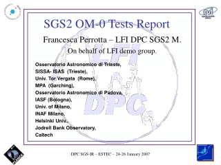
1. SGS2 OM-0 Tests Report Francesca Perrotta – LFI DPC SGS2 M. On behalf of LFI demo group. Osservatorio Astronomico di Trieste, SISSA- ISAS (Trieste), Univ. Tor Vergata (Rome), MPA (Garching), Osservatorio Astronomico di Padova, IASF (Bologna), Univ. of Milano, INAF Milano, Helsinki Univ., Jodrell Bank Observatory, Caltech

2. Goal: make the SGS2 Pipeline commensurate with Planck scientific objectives. • Verification plans are being followed • Scientifical performances assessed on the basis of tests on prototypes.

3. Goal: make the SGS2 Pipeline commensurate with Planck scientific objectives. • Verification plans are being followed • Scientifical performances assessed on the basis of tests on prototypes. ---------------------------------------------------------------------- • Integration status and improvements w.r.t. previous status (D. Maino) • Operation planning (A. Gregorio) • Pipeline tests results (F. Perrotta) [Reference: PL-LFI-OAT-RP–015,“Planck LFI- SGS2 End-to-end test report” ] ----------------------------------------------------------------------

4. Baccigalupi C. (SISSA), Balbi A. (Tor Vergata University, Roma) Banday A. (MPA Garching), Bersanelli M. (Milano Univ.), Bonaldi A. (OAPd), Burigana C. (IASF Bologna), Cappellini B. (Milano Univ.), Danese L. (SISSA), De Gasperis G. (Universita’ Tor Vergata, Roma) , De Zotti G. (Padova Observatory), Donzelli S. (Milano Univ.), Facchinetti S. (INAF Milano), Finelli F. (IASF Bologna), Gasparo F. (OAT), Gonzales-Nuevo J. (SISSA), Gruppuso G. (IASF Bologna), Keihanen E. (Helsinki Univ.), Kurki-Suonio H. (Helsinki Uni.) , Leach S. (SISSA), Leahy P. (Jodrell Bank Observatory), Lenardon L. (INAF Milano), Mandolesi N. (IASF Bologna), Massardi M. (SISSA), Mennella A. (Milano University), Natoli P. (Universita’ Tor Vergata, Roma), Pasian F. (OAT), Perrotta F. (OAT), Platania P. (Milano Univ.), Poutanen T. (Helsinki Univ.), Reinecke M. (MPA Garching), Rocha G. (Caltech), Sandri M. (IASF Bologna), Stivoli F. (SISSA), Stringhetti L. (IASF Bologna), Tomasi M. (INAF Milano), Villa F. (IASF Bologna), Zacchei A. (OAT) (LFI demo group) Solid team of people involved in validation plan:

5. Strict link between scientific production and data analysis Baccigalupi C. (SISSA), Balbi A. (Tor Vergata University, Roma) Banday A. (MPA Garching), Bersanelli M. (Milano Univ.), Bonaldi A. (OAPd), Burigana C. (IASF Bologna), Cappellini B. (Milano Univ.), Danese L. (SISSA), De Gasperis G. (Universita’ Tor Vergata, Roma) , De Zotti G. (Padova Observatory), Donzelli S. (Milano Univ.), Facchinetti S. (INAF Milano), Finelli F. (IASF Bologna), Gasparo F. (OAT), Gonzales-Nuevo J. (SISSA), Gruppuso G. (IASF Bologna), Keihanen E. (Helsinki Univ.), Kurki-Suonio H. (Helsinki Uni.) , Leach S. (SISSA), Leahy P. (Jodrell Bank Observatory), Lenardon L. (INAF Milano), Mandolesi N. (IASF Bologna), Massardi M. (SISSA), Mennella A. (Milano University), Natoli P. (Universita’ Tor Vergata, Roma), Pasian F. (OAT), Perrotta F. (OAT), Platania P. (Milano Univ.), Poutanen T. (Helsinki Univ.), Reinecke M. (MPA Garching), Rocha G. (Caltech), Sandri M. (IASF Bologna), Stivoli F. (SISSA), Stringhetti L. (IASF Bologna), Tomasi M. (INAF Milano), Villa F. (IASF Bologna), Zacchei A. (OAT) (LFI demo group) Solid team of people involved in validation plan:

6. The SGS2 LFI Om-0- capabilities • Instrument parameters reconstruction: computes the R gain modulation factor for each detector and determine the noise parameters (knee frequency, slope of the 1/f noise component, white noise NET) for each detector, together with an estimate of the relative errors. • Photometric Calibration: determines the calibrationconstant(s). Calibration is performed both on short timescales to monitor the instrument stability, and on long timescales to provide an accurate “absolute” calibration. • Pointing and beam reconstruction: reconstructs the pointing of each detector given the Spacecraft pointing, and obtain maps of the main beam patterns for each feed-horn. • Single channel and frequency map making: map making tools are used to produce single channel maps and final optimal combination maps.

7. The SGS2 LFI Om-0 - blocks Main sub-pipelines: 2 4 3 1

8. Towards Phase I of End-to-end Tests • Only temperature processing requested by Phase I definitions. However, we could make use of polarization simulated data too; • the sky model is based on the “concordance model” CMB (no non-gaussianity); • the dipole does not include sub-modulations due to Lissajous orbit around L2; • the Galactic emission obtained assuming non-spatially varying index; • non-idealities in the instrumental properties are not included: the detector model is “ideal” and does not vary with time; • the scanning strategy (baseline Level S) is “ideal” (no gaps in the data); however, we were able to use realistic feed horn beam patterns, though the patterns are assumed constant within the bandwidth.

9. Test procedures - generalities The execution of Phase I OM-0 tests performed in parallel: specific inputs are provided to be used in a single test. The four main blocks of processing have been tested through individual ProC sub-pipelines. For each test are given: • Detailed test objectives; • Participants; • Definition of simulations; • Specs. on the input data to DPC • Hardware and infrastructure to run the tests • Specs. of the tests outputs (list of parametersXi) • I/O comparison: • Dx =xs-xm and er=em/x • (Figures of merit PASS/FAIL CRITERIA)

10. Tests platform (hardware, libraries, formats) • SGS2 Pipeline installed on the Beowulf system OAT. Actual LFI DPC resources: 44 CPUs with a total of 38 GB of RAM and 2.2 TB of disk space. The DPC uses the PBS queueing system. We use the following queues: planck: 18 node x 2 processors (18 Intel Pentium III) fast: 4 node x 2 processors (4 Opteron Dual Core). • Individual Pipeline units are Fortran 90 and C++ modules. Also used MPI parallel codes interface. External libraries included: FITSIO and FFTW . • Inputs files for tests are FITS files; all the Pipeline procedures compatible with the LFI TOI DPC format and with the MPA-DMC fits implementation. The use of the MPA-DMC will be simply inserted just recompiling the SGS2 pipeline with the appropriate libraries. The LFI DPC is actually ingesting the data into the database.

11. Input data (simulations) LFI-demo simulated 12 months (8784 rings) time streams for the two horns of the 30 GHz channel (LF 27 and LFI 28), two radiometers each. All the simulations generated on the Beowulf system, at the OAT. The TODs are in FITS format (with nside nside=2048, 1’ resolution) and include: • the 30 GHz reference sky (noiseless CMB from WMAP data; galactic emission from synch., free-free, dust, thermal SZ). The dipole components are added during the TODS production; • bright point sources (radio + IR) and planets; (The radio sources are constrained simulations using WMAP data, and the NVSS, SUMMS and PMN surveys. IR basically from IRAS) • two independent realizations of white noise; 1/f noise Optics: Main beams have been computed with GRASP9, propagating the measured pattern of the feed horns #27 and #28 through the ideal telescope. The focal plane database file has been modified, according to the values obtained during the FM RCA test campaign. Scanning strategy: baseline

12. R factor Inputs (produced at Level S in the actual LFI TOI DMC): -Signal TOI (diffuse em., tot. dipole,bps)+ wn(1) -TOI from nominal wn params; convolved with 30 GHz beam. -Reference TOI (Tload = 4.5 K) +wn(2) The pipeline generates R by averaging over 1 hr of obs. sky and load signals, for each radiometer.

13. R factor NOTE: accuracy on the reconstruction of R not fully representative of that achievable during flight. Uncertainty in R dominated by the total 1/f noise in sky and load signals. This was not generated for this test.

14. Noise properties I • After R determination, the pipeline creates differential data stream as DV=Vsky–RVload. A realization of 1/f residual noise TOI is added to DV. The total time stream is given as input to noise_ps which produces the resulting noise power spectrum. • From the noise power spectrum, Fitnoise_GT estimates the white noise limit, knee frequency f* and slope a, as well as the relative errors. • PS on 1 hr data, 24 hr data, and on the average of 24 hr data. • 1 hr Spectra obtained by averaging over 24 cycles in a day.

15. Noise properties II Estimated power specrum of signal + noise

16. Noise properties III Noise Power spectrum after removal of signal estimate. (Destriping is first applied; resulting map is re-observed according to pointing parameters).

17. Rel. errors on noise params.

18. Beam reconstruction I Provides a parameterised model of the Planck-LFI beams and an estimate of the focal plane geometry based on LFI data alone (initial guess of the FP geometry is assumed based on the knowledge from instrument integration phase).The beam response averaged over the bandwidth is approximated as: The beam shape in the x-y plane is described by a bivariate Gaussian: where and

19. OUTPUTS: x,y (coordinates of the main beam on the focal plane); a (orientation of the beam, i.e. anti-clock rotation angle of the elliptical bivariate Gaussian w.r.t. the x field of view axis); s beam = e Beam reconstruction II S/C pointing FP geom. LFI 30 GHz horns Gdestri beamfit Beam params. I/O comparison: we computed the (r.m.s.) reconstruction sensitivity (Dx) for each parameter. The error in each specific realization is in good agreement with the quoted sensitivity.

20. Beam reconstruction III Same precision for detector #28

21. Map making Maps for the single n channels, using the whole detectors data set. Two approaches have been used: • Madam, based on the destriping technique + infos on the noise spectrum in the form of a noise filter. The low-frequency noise component is modelled as sequence of constant offsets or 'baselines‘ determined by maximum likelihood analysis. The baseline length is an adjustable input parameter. The baselines are subtracted from the TOD, and the remaining TOD is binned into a map. • Roma, GLS map making code. ROMA maps are “optimal” (minimum variance; built taking into account exact pixel-pixel covariance) Simulations: • Signal = CMB+synchrotron+dust+free-free+faint point sources+ SZ • 12 months TODs for the four LFI 30 GHz detectors. Cycloidal scanning. • Asymmetric beams. • Perfect calibration, dipole removal and R factor. • All maps are Nside 512.

22. Map making- MADAM results Three destriping methods were used: A. 1 hour baselines, standard mode, noise filter OFF B. 1 min baselines, split-mode, noise filter OFF C. 1.2 sec baselines, split-mode, noise filter ON In standard mode all data are processed simultaneously. In split-mode, data are processed in pieces, 2 months at a time. The optimal map-making method (1.2 sec baselines, standard mode, noise filter ON) couldn’t run on the present Beowulf configuration. • Noise filter parameters: f knee = 0.05 Hz; f min = 1.15e-5 Hz; slope a = -1.7. White noise level is not needed. • Madam makes no assumptions about beam shape. Output map includes smoothing by the beam. • The code outputs the map in the units of the TOD.

23. Map making- MADAM results Madam output: 30 GHz Temperature map

24. Madam output: 30 GHz U and Q map

25. Madam - Residual maps(output – binned noiseless)

26. Q, U RESIDUAL MAPS – Nside 512 – MADAM, 1 min baselines R-J mK R-J mK

27. Madam- Angular Power Spectra Power spectra of the CMB, signal plus noise, smoothed reference, signal bin and residual (noisy output-binned noiseless map). 1 min baseline. Horizontal dashed line: expected spectrum of the white noise

28. Polarization analysis: Q and U angular power spectra of the CMB, signal plus noise, smoothed reference, signal bin and residual (noisy output map and the binned noiseless map). 1 min baseline. The horizontal dashed lines indicate the expected spectrum of the white noise. Angular Power Spectra - MADAM

29. Temperature analysis Madam vs. ROMA-Angular Power Spectra of Residual Maps.

30. Polarization analysis Madam vs. ROMA-Angular Power Spectra of Residual Maps. EE and BB cross spectra

31. Madam- 1hr baseline Residual 1/f - Madam vs. Roma 1) Residual: ClXX = spectrum of the residual map sT,Q,U = theoretical rms of white noise map 2) White noise: 3) Residual 1/f: ClXX = difference of above two spectra

32. Madam vs. ROMA- Residual maps Rms Baselines 1 houra 1 mina 1.2 secb MADAMMap Rms Map RMS Map RMS White theoreticalc T 34.58 32.6832.57 32.45 Q 48.81 46.1846.02 45.83 U 49.30 46.6246.45 46.26 ROMAb T 33.21 Q 46.90 U 47.38 Units are mK (R-J @ 30 GHz). a – without noise filter b – with noise filter c – White noise RMS is derived from the block diagonal approximation of the pixel-pixel noise covariance.

33. Open areas • We performed the tests for the 30 GHz LFI channels, from simulated TODs up to single channel and frequency maps. Same has to be done for the other channels. • Test calibration sub-pipeline • Realistic estimate of R (total power 1/f noise included) • The extraction of the astrophysical and cosmological informations from these outputs (the “Level 3” of Data Processing), requiring the separation of the CMB signal from foregrounds emission, is a high-priority target. Mostly important for Polarization. • Perform tests with serial execution with the use of ProC+DMC with DB as back end • e2e Tests should be completed byend of May 2007 • Straylight effects (Phase II ?)

34. Conclusions • Verification plans are being followed; • internal tests show that the SGS2 OM-0 LFI DPC Pipeline is actually able to reconstruct the main “Phase-I” parameters up to a quite good precision level; • open areas clearly identified; • schedule for main targets established; • limitations imposed by CPU power should not be an issue; • data processing and Scientific competences are closely linked in the actual LFI SGS2 team structure; • team management proceeding smoothly; • Interface HFI/LFI being implemented in the Operation Plan; effort is being produced in clarify how the SGS2 Pipeline will be operated.