Exponential functions

1. Exponential functions

2. Information

3. Introducing exponential functions What can you say about this function? Is it increasing or decreasing? y Does it have a constant rate? x Does it have any maxima or minima? How does it behave at either end? How do you think this function is written?

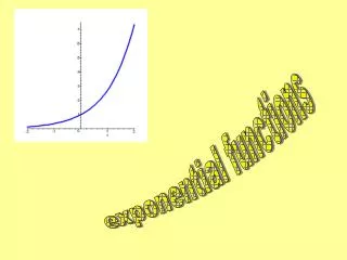
4. Exponential functions An exponential function is a function in the form: where a is a positive constant. y= ax Here are examples of three exponential functions: y = 2x y = 3x y = 0.25x In each of these examples, the x-axis forms an asymptote.

5. Exploring exponential graphs

6. Summary of graphs When 0 < a < 1, the graph of y = ax has the following shape: y (1, a) (1, a) x The general form of an exponential function base a is: f(x) = ax where a > 0 and a≠1 When a > 1, the graph of y = ax has the following shape: y 1 1 x In both cases the graph passes through (0, 1) and (1, a). Why does this happen?

7. Introducing exponential growth Exponential growth occurs when the amount a quantity increases by is proportional to its size. The larger the quantity gets, the faster it grows. Quantities that grow exponentially include: • investments with a fixed compound interest rate, • the number of microorganisms in a culture dish, • population size.

8. Introducing exponential decay Exponential decay occurs when the amount a quantity decreases by is proportional to its size. The smaller it becomes, the more slowly it decays. Quantities that decay exponentially include: • the rate at which an object cools • the number of atoms in a radioactive isotope • the value of a car as it depreciates.

9. Exponential growth example A population of 100 bacteria doubles in size every minute. Write a function to model the growth of the bacteria. We can write the values for the first few minutes in a table: time (mins) 0 1 2 3 … t number of bacteria 100 200 400 800 … 100 × 2t = 100 × 4 = 100 × 8 = 100 × 2 = 100 × 2² = 100 × 2³ N = 100 × 2t If N is the number of bacteria after t minutes, then: More generally, if N0 is the number of bacteria when t = 0, N = N02t

10. Linear and exponential

11. Compounding interest problems

12. Compounding interest

13. The number e This number denoted by e is an irrational number. e = 2.718281828459045235… (to 19 significant digits) Most scientific calculators have ex as a secondary function above the key marked “ln”. The function ex is called the exponential function or the natural exponential. This is not to be confused with an exponential function, which is any expression of the general form ax, where a is a constant.

14. Transformations of f(x) = ex

15. Exponential growth function y In general, exponential growth can be modeled by the function: y = y0ekt y = y0ekt • t is time • y0 is the original quantity (the quantity when t = 0) • y is the quantity after time t • k is a positive constant (the growth rate) y0 • the domain is 0 ≤ x < ∞ 0 t • the range is y0≤ y < ∞.

16. Exponential decay function y In general, exponential decay can be modeled by the function: y = y0e–kt • t is time • y0 is the original quantity (the quantity when t = 0) • y is the quantity after time t y0 y = y0e–kt • k is a positive constant (the decay rate) • the domain is 0 ≤x < ∞ 0 t • the range is 0 < y≤y0.

17. Exponential decay example The mass of a sample of radioactive iodine, m grams, decays according to the formula: where t is the number of days after it is first observed. a) What is the initial mass of the sample? b) Sketch the graph of m against t. c) What is the mass of the sample after 2 days?

18. Exponential decay solutions m 15 t a) What is the initial mass of the sample? When t = 0, m = 15e0 = 15 The initial mass of the sample is 15g. b) Sketch the graph of m against t. The graph of m = 15e–0.083t will be an exponential decay curve passing through the point (0, 15). c) What is the mass of the sample after 2 days? When t = 2, m = 15e–0.083 × 2 = 12.71 (to the nearest hundredth) The mass of the sample after 2 days is 12.71g.