High-throughput RNAi screen morphologic analysis
High-throughput RNAi screen morphologic analysis. Gregoire Pau, Oleg Sklyar, Remy Clement, Wolfgang Huber EMBL-EBI Cambridge Florian Fuchs, Christoph Budjan, Thomas Horn, Michael Boutros DKFZ Heidelberg. Experimental setup. Genome-wide RNAi knockdown (~17000 genes)

High-throughput RNAi screen morphologic analysis
E N D
Presentation Transcript
High-throughput RNAi screen morphologic analysis Gregoire Pau, Oleg Sklyar, Remy Clement, Wolfgang Huber EMBL-EBI Cambridge Florian Fuchs, Christoph Budjan, Thomas Horn, Michael Boutros DKFZ Heidelberg
Experimental setup • Genome-wide RNAi knockdown (~17000 genes) • HeLa cells, incubated for 48h • Microscopy readout: DNA (DAPI) ,Tubulin (Alexa) , Actin (TRITC) wt- wt- wt- BTDBD3 CEP164 CD3EAP
Goal • Biological question: • What are the most striking phenotypes in the screen ? • What are the genes KD giving rise to the same phenotype ? • Which should be understood as: • Given a phenotypic distance • What are the farthest phenotypes from the negative controls ? • What are the genes KD giving rise to close phenotype ?
Phenotypic distance • What are the phenotypes which are close/distant ? How to deal with the natural phenotype large variability ? wt- wt- wt- BTDBD3 CEP164 CD3EAP
Gene phenotype • Not a cell phenotype ! • Quantitative phenotypic profile expressed by a population of cells: • Number of cells • Mean cell features (size, eccentricity, …) • Cell classes distribution (normal, mitotic, condensed, protruded…) • A distance will be then defined between phenotypic profiles CEP164 CD3EAP
Beyond cell classes ? • Cell features distribution • Using a probabilistic model ? • Defining classes = assuming "hard" boundaries Cell feature 2 (X*2) Cell feature 2 (X*2) Cell feature 1 (X*1) Cell feature 1 (X*1) O Interphase O Metaphase O Debris
imageHTS • R package • Able to compute the phenotype profile of an image • Works for our screen, generalization needs to be worked out • Open-source free software • To be released (soon) • Rely on the R package EBImage • Low-level basic image processing • Available on Bioconductor
Workflow Image Segmentation Cells Features extraction Cells features Classification CEP164 Cell phenotypes Intensity = 1778 Cell size = 421 Eccentricity = 1.08 Actin.intensity = 124 Tubulin.intensity = 94 DNA.intensity = 74 Nucleus.size = 46 Actin.hz11 = 17.4 Actin.hz12 = 11.3 Tubulin.hz11 = 8.4 Tubulin.hz12 = 7.5 Nucleus.hz11 = 3.4 ... Metaphase Phenoprinting ~30 secondes/well ~10 days/CPU/genome Gene phenotype
Segmentation • Goal: how to isolate cells from an image ? • Which means: how to 'explain' to a computer what a cell is Cells are 2D connected sets. Cell boundaries are delimited by a Tubulin cytoskeleton and maybe some actin protusions. Cells contains at least one nucleus. Cell size is bounded. A nucleus cannot be bigger than the cell and has a bounded size. Z = A + T Nmask = (H - Hm) > t1 Cmask = (Zn > t2) t2 must fulfill (Tn > v) Cmask & (An >v) Cmask …
Segmentation • Result • Accurate results if cells are not too packed • Superposition is tricky to handle !
Cell features • Goal: how to characterize a cell in terms of numerical values ? • Cells exhibit a lot (too much) of morphological changes: • Size, eccentricity, angle • Position in the well • Shape (rugged, smooth…) • Actin intensity • Tubulin spatial distribution • … • What are the interesting cell features ? • Depends on the biological question • Need for rotation, symmetry, translation invariance • Need for quantitative features !
Cell features • Examples
Cell features • Examples Cell size = 482 Nucleus size = 171 Nucleus perimeter = 98 Cell eccentricity = 1.1 Actin spatial w00 = 1.73 … (50 in total: many more about actin distribution, tubulin granularity, actin fibers…) Each cell is now characterized by a vector of 50 num. features
Classification • Goal: how to classify a cell given its features ? • Supervised learning using SVM • Using 8 classes and a training set of ~3000 cells: Actin Fiber Lamellipodia Big cells Metaphase Condensed Normal Debris Protusion Cells in these classes are expected to have similar features
Classification • Result • Classification performance (5-fold CV) on TS: ~85 %
n int ext ecc AtoTint Next Nint NtoATsz AF BC C D LA M MB N P Z 78 924.14 28.11 0.7121 0.745 11.01 393.12 0.341 3 6 9 19 11 3 9 17 5 4 Gene x How to compute a distance between heterogeneous traits ? Phenotypic profile • Expressed by a population of cells CEP164 n int ext ecc AtoTint Next Nint NtoATsz AF BC C D LA M MB N P Z 128 1054.74 25.56 0.6491 0.720 12.752 373.28 0.237 2 7 32 15 0 17 2 45 6 2 CEP164
Gene phenoprint • Goal • Cut off the variability of the phenotypic traits • Keep only the significant trends • Assuming that phenotypic traits are binary • Use of a parametric sigmoid transform • Each phenotypic trait is mapped to [0,1] • Boring zone [0,0.5] • Red: significant increase • Blue: significant decrease • How the parameters , can be determined ? • For 7*2 (both) + 6 (inc) = 20 different phenotypic traits !
Distance learning • Ideas: • KD of pairs of interacting genes may lead to similar phenotypes • Distance of gene pairs picked on STRING should be lower in average than two random gene pairs • Distance learning • Let D+ the set of all pairwise gene distances picked on STRING • Let D- the set of all pairwise gene distances picked randomly • Goal: find the parameters k and k that best separate D+ and D-
Gene phenoprints • Definition • Raw phenotypic profiles • Sigmoid transformed with an optimized set of parameters • L1 distance between gene phenoprints • Informative metric • To discover extreme phenotypes (distant from negative controls) • To discover close phenotypes • Hits • Contains a non-zero pheno. trait • 1891 hits (among 22839)
Discovering extreme phenotypes • Condensed phenotype • Elongated STK39 STK39 TENC1 LOC51693 KCNT1 LOC51693 KCNT1
Discovering extreme phenotypes • Binucleated • Large cells phenotype ADRB2 KIAA0363
EBImage • Set of quantitative image processing tools • Image IO, displaying • Filtering • Morphological operators • Goal • Low-level tools • Can be used as building blocks • To 'translate' a biological question into a model/algorithm • Ex: what is a cell ? • Some examples • Low-pass filter, high-pass filter, thresholding
Image representation • Raster/bitmap representation • Matrix of numbers ranging from 0 (black) to 255 (white) 105 67 51 42 35 31 28 26 27 27 85 59 46 41 36 31 30 28 32 29 67 53 43 40 35 31 31 33 37 29 59 50 42 39 37 33 34 39 39 31 54 50 42 38 37 36 39 48 41 34 51 45 42 40 37 36 43 54 43 32 48 45 42 42 38 44 48 54 41 36 47 42 47 42 44 52 56 51 41 36 45 44 44 44 50 59 60 50 41 35 46 45 44 47 59 60 59 45 39 33 83 56 46 39 33 30 27 26 27 24 65 51 44 38 33 32 28 29 30 22 56 49 41 37 35 33 31 35 34 25 55 45 40 37 33 33 36 43 37 25 50 42 41 38 37 36 41 47 38 28 47 44 42 40 37 39 49 46 39 29 46 43 40 40 40 48 53 43 36 33 45 43 41 44 44 55 57 45 35 32 45 42 42 45 54 58 53 44 38 31 47 46 46 54 63 62 49 44 37 31 ...
Color representation • RGB color representation: 1 image for each channel Red channel (here, Actin) Green channel (Tubulin)
Color representation • RGB color representation: 1 image for each channel Blue channel (DNA) Combined
Linear filter • Low-pass filter x 1 1 1 1 1 1 1 1 1 x Can be used to wipe noisy/small uninteresting details
Linear filter • High-pass filter x -1 -1 -1 -1 8 -1 -1 -1 -1 x Useful to detect cell edges
Thresholding • Global thresholding x x > 25 Useful to isolate cells
Goal "How two gene phenotypes are close together ?" How to define close ? ? ? Gene 1 ? Gene 2 Gene 3
Distance • Assuming • Each gene i is described by a set of p descriptors • Distance d between gene i and j is parametric • Example • xik is the k-phenotype cell count observed on gene i • Weighted L2 distance: • Sigmoid-transformed coefficients + weighted L1 distance: • How to choose the parameters k,k and k?
Minimizing over STRING • STRING is a pairwise gene interactions database • Idea: distance of genes picked on STRING should be lower in average than two random genes • Idea • Let D+ the set of all pairwise gene distances picked on STRING • Let D- the set of all pairwise gene distances picked randomly • Goal: find the parameters k, k and k that minimize D+ while maximizing D- • Target criterion to minimize : z' score between D+ and D-, to maximize their separability
Results • After hundred of iterations using BFGS with optim • Z' went down from -4.32 to -2.11
Caveat • Target function is not smooth and hard to optimize • Smoothing is needed during optimization !