Forecasting Federal Funds Rate Changes Using Financial Indicators
Explore how GDP, CPI, and stock market prices impact Fed funds rates. Develop models to forecast future rates and interpret economic implications. Utilize data analysis and statistics to predict changes in interest rates accurately.

Forecasting Federal Funds Rate Changes Using Financial Indicators
E N D
Presentation Transcript
Forecasting Fed Funds Rate Group 4 Neelima Akkannapragada Chayaporn Lertrattanapaiboon Anthony Mak Joseph Singh Corinna Traumueller Hyo Joon You
Background • Fed funds rate (FFR) as an instrument of control. • FFR as sign of economic strength/weakness. • FFR is at 1.25%, the lowest since 1961. • Greenspan intimates at possibility of deflation (last week). • Japanese Deflation and the Great Depression.
Objectives • What will happen to the FFR given indicators such as GDP, CPI, stock market price levels, etc? • Create a distributed lag model with FFR as the dependent variable. • Provide one period ahead forecast of FFR. • And what does this forecast mean to us? • Provide economic context for the forecast.
The Idea • Supposing that the Fed made its decision solely on previous FFR would be naive. • Fed’s decision on future FFR depends on existing information. • We focus on these existing information to explain FFR. • GDP • CPI • SP500
Data Standardization • All data from Fred II. • Different time range and frequencies • But same time range and frequencies necessary for DL model • Lower bound set by data with the latest start (SP5000 Jan 1970) • Upper bound set by data with the earliest end (GDP Jan 2003) • Frequency set by data with lowest frequency (GDP quarterly). • Result is a shorter and less frequent data set (120 obs). • Still enough data.
Time Causality Pairwise Granger Causality Tests Date: 05/27/03 Time: 14:23 Sample: 1970:1 2003:2 Lags: 2 Null Hypothesis: Obs F-Statistic Probability DLGDP does not Granger Cause DLFFR 130 12.8145 8.7E-06 DLFFR does not Granger Cause DLGDP 1.75070 0.17788 DLSP does not Granger Cause DLFFR 130 7.35499 0.00096 DLFFR does not Granger Cause DLSP 2.07473 0.12989 DDLCPI does not Granger Cause DLFFR 129 0.61862 0.54034 DLFFR does not Granger Cause DDLCPI 7.36316 0.00095 DLSP does not Granger Cause DLGDP 130 1.16482 0.31534 DLGDP does not Granger Cause DLSP 0.54295 0.58240 DDLCPI does not Granger Cause DLGDP 129 3.40096 0.03648 DLGDP does not Granger Cause DDLCPI 2.80740 0.06420 DDLCPI does not Granger Cause DLSP 129 1.48890 0.22963 DLSP does not Granger Cause DDLCPI 0.48034 0.61972
Estimation Output DL Model Dependent Variable: DLFFR Method: Least Squares Sample(adjusted): 1972:2 2003:1 Included observations: 124 after adjusting endpoints Convergence achieved after 8 iterations Variable Coefficient Std. Error t-Statistic Prob. C -0.17718962391 0.0332222708495 -5.33345913387 4.6565699798e-07 DLGDP(-1) 5.74253059866 1.3480009163 4.26003464036 4.10881431448e-05 DLGDP(-3) 3.12720392868 1.31542817995 2.37732776016 0.0190325621418 DLSP(-1) 0.429515053545 0.162069622027 2.65018853116 0.00913844465895 AR(5) 0.246953114484 0.0878659566173 2.8105665037 0.00578442215627 R-squared 0.27792384769 Mean dependent var -0.00836815797483 Adjusted R-squared 0.253652380385 S.D. dependent var 0.15270778165 S.E. of regression 0.13192640994 Akaike info criterion -1.17365786942 Sum squared resid 2.07114473911 Schwarz criterion -1.05993683855 Log likelihood 77.766787904 F-statistic 11.4506405485 Durbin-Watson stat 1.79038035224 Prob(F-statistic) 6.75508422109e-08 Inverted AR Roots .76 .23+.72i .23 -.72i -.61 -.44i -.61+.44i
Summary • Standardization of data for DL modeling causes results in fewer observations. • Granger test is useful in isolating independent variables. • dlSP500 did not have AR structure. Creating the transformed dependent variable may have been more difficult. • Result is more plausible than ARMA model. • Fed funds rate will go down next quarter.
What Now? • Assuming that fed funds will continue to go down, one can… • buy treasury bonds now and sell them later at a higher price when interest rate drops • simply try harder to find a job in the sluggish economy • start a business now in anticipation of next boom
Estimation Output AR Model Dependent Variable: DLFFR Method: Least Squares Sample(adjusted): 1970:3 2003:1 Included observations: 131 after adjusting endpoints Convergence achieved after 3 iterations Variable Coefficient Std. Error t-Statistic Prob. C -0.014695 0.016465 -0.892533 0.3738 AR(1) 0.166843 0.088232 1.890959 0.0609 R-squared 0.026971 Mean dependent var -0.014326 Adjusted R-squared 0.019428 S.D. dependent var 0.158538 S.E. of regression 0.156991 Akaike info criterion 0.850112 Sum squared resid 3.179341 Schwarz criterion -0.806216 Log likelihood 57.68233 F-statistic 3.575725 Durbin-Watson stat 1.961340 Prob(F-statistic) 0.060873