Download
1 / 23
230 likes | 330 Views
DESY BT analysis - Systematics summary -. S. Uozumi Dec-5 th 2011 ScECAL meeting. sources and evaluation method of systematics (based on data). Perform pseudo-experiments and see variation Response calibration by MIP (stat. uncertainty of calib. const)

E N D
DESY BT analysis- Systematics summary - S. Uozumi Dec-5th 2011 ScECAL meeting
sources and evaluation method of systematics(based on data) Perform pseudo-experiments and see variation • Response calibration by MIP (stat. uncertainty of calib. const) • Correction for temperature dependence (stat. uncertainty of temperature-gain correction coefficient) Take edge-to-edge width : • Light cross-talk (on and off) • MPPC saturation correction • MPPC gain measurement by LED system (stat error of 1 p.e. signal) • Electronics inter-calibration of low/high gain modes (uncertainty of inter-calib factor) • Shape of saturation correction curve (effective num. of pixels)
Systematics from MIP calibration Distribution of calib constant and its statistical uncertainty for all the channels of 3 configurations :
Systematics on MIP calibration Result of 100 pseudo-experiment (DRMS/RMS = 7%) : Deviation from Linearity Energy resolution
Systematics on MIP calibration summary • Effect is comparable or smaller than stat. uncertainties. • Relatively large effect on resolution of 3rd configuration.
Systematics on temp. correction Calib. Const. (ADC counts) From CAN-006 : Temperature (oC) Distribution of temp. correction factor and its statistical uncertainty for all the channels of 3 configurations :
Systematics on temp. correction Result of 100 pseudo-experiment (DRMS/RMS = 7%) : Deviation from Linearity Energy resolution
Systematics on temp. correction summary • Effect is comparable or slightly larger than stat. uncertainties.
Systematics on Light cross-talk • Compare results with cross-talk correction turned on/off, and double. • No much effect except 3rd config quarter region.
Systematics on Light cross-talk • Compare results with cross-talk correction turned on/off, and double. • A clear change on constant term with 3rd config central region, thinking why… • No much effect for others.
Systematics on saturation correction (1) • Signal in ADC counts is converted to num. of fired pixels to apply MPPC saturation correction. • d-values = ADC counts for 1 p.e. (see reference) obtained with LED gain measurement system: dlow-gain [ADC counts] = dhigh-gain / Cinter = 14.4 +- 1.5 for fiber readout module 15.8 +- 1.6 for direct readout module 18.1 +- 1.9 for fiber readout module • Note that only ~5% of whole channels have LED system at DESY BT. • ~10% uncertainties, mainly come from inter-calibration factor. Vbias = 76.75 V dhigh-gain= 206.9
Systematics on saturation correction (1) • Change dlow-gain for + one standard deviation of and compare results. • No much effect among all.
Systematics on saturation correction (1) • Change dlow-gain for + one standard deviation of and compare results. • Some amount of effect, which is not negligible.
Systematics on saturation correction (1) • Saturation curves were measured for each of 3 configurations after the beam test (see reference for detail) Npix = “effective” number of pixels x = ADC / dlow-gain Npix = 2072.8 (fiber readout) = 1677.2 (direct readout) = 2270.5 (extruded)
Systematics on saturation correction (2) • Just take two extreme cases, change Npix for all the configurations : Npix = 1600 (assume no enhancement of Npix) or 2270 • This source dominates overall uncertainty on deviation.
Systematics on saturation correction (2) • Just take two extreme cases, change Npix for all the configurations : Npix = 1600 (assume no enhancement of Npix) or 2270 • Effect is non-negligible.
Deviation including all uncertainties • We can say “Linearity is confirmed to be within + 2%”.
Resolution – plot ONLY stat. uncertainty • Same with one what we already have in CAN-012. • Systematics must be added in terms of sstat and sconst .
Resolution statistical and systematic uncertainties • Systematics from MIP calibration and temp. correction are small enough, while others gives effects of order 0.1 ~ 1 %.
Summary • Plots and tables on systematics study are being finalized. • Dominant uncertainty on deviation comes from uncertainty of effective num. of MPPC pixels, but still deviation stays within +2%. • For resolution, cross-talk and saturation correction are dominant on systematics. • Issues & to-do list: • Are evaluation method all correct ? • Behavior of 3rd config module on x-talk correction (page 10) – why? • Npix region is reasonable ? • Systematics from strip response non-uniformity ? • CALICE note for systematics. • Paper draft – version 0.5 ready for revision up to section 3. Working on other sections.
==> sys_temp.systxt <== • 2 0 0 0.0229901 -0.0229901 0.00844141 -0.00844141 • 2 1 0 0.0122069 -0.0122069 0.0222885 -0.0222885 • 2 2 0 0.0939667 -0.0939667 0.0409135 -0.0409135 • 3 0 0 0.0417832 -0.0417832 0.0170234 -0.0170234 • 3 1 0 0.0164397 -0.0164397 0.0158716 -0.0158716 • 3 2 0 0.0410246 -0.0410246 0.0515202 -0.0515202 • ==> sys_xtalk.systxt <== • 2 0 0 0.0376001 -0.0612989 0.27904 -0.29048 • 2 1 0 0.101301 -0.074099 0.0636995 -0.0302803 • 2 2 0 0.202399 -0.0134006 0.65127 -0.76918 • 3 0 0 0.1592 -0.080201 0.22214 0 • 3 1 0 0.0534996 -0.00880063 0.40214 -0.0551302 • 3 2 0 0.0259995 -0.00279993 0.41221 0 • ==> sys_MIP.systxt <== • 2 0 0 0.0095387 -0.0095387 0.0212333 -0.0212333 • 2 1 0 0.0133516 -0.0133516 0.022889 -0.022889 • 2 2 0 0.0680983 -0.0680983 0.0577163 -0.0577163 • 3 0 0 0.0184793 -0.0184793 0.016356 -0.016356 • 3 1 0 0.0164871 -0.0164871 0.0167485 -0.0167485 • 3 2 0 0.0286047 -0.0286047 0.0409721 -0.0409721 • ==> sys_Npix.systxt <== • 2 0 0 0.0527009 -0.2417 0.62048 -0.15401 • 2 1 0 0.0725001 0 0.00740997 -0.26662 • 2 2 0 0.0048995 -0.5437 0.65224 0 • 3 0 0 0.059098 -0.530101 1.09924 -0.19962 • 3 1 0 0.0734001 -0.00990033 0.0232298 -0.28046 • 3 2 0 0 -0.09 0.44967 0 • ==> sys_dval.systxt <== • 2 0 0 0.0347003 -0.0764996 0.2186 -0.1408 • 2 1 0 0.0211 -0.0444993 0.118089 -0.09447 • 2 2 0 0.2212 -0.1128 0.17426 -0.18035 • 3 0 0 0.0764996 -0.129502 0.34429 -0.24733 • 3 1 0 0 -0.0421003 0.10988 -0.0535503 • 3 2 0 0.011 -0.0364006 0.0818001 -0.04023
Pseudo-experiment overview • Applicable for systematics from MIP calib. and temperature correction. • Just randomly change parameter channel-by-channel, and perform pseudo-experiments. • See variation (RMS) in terms of resolution and linearity. • How many pseudo-experiments? Assuming variation follows Gaussian distribution, uncertainty of variation is (N = num. of pseudo-experiments) For a moment, take N=20 Which gives “uncertainty of uncertainty” of ~16 %.