Download
1 / 48
510 likes | 746 Views
Physical oceanography, tides and coastal flooding – the science behind it all. Dr Kevin Horsburgh Head of the National Tidal and Sea Level Facility Physics Teachers Conference 26 June 2008. Proudman Oceanographic Laboratory.

E N D
Physical oceanography, tides and coastal flooding – the science behind it all Dr Kevin Horsburgh Head of the National Tidal and Sea Level Facility Physics Teachers Conference 26 June 2008
Proudman Oceanographic Laboratory • Is a component laboratory of the Natural Environment Research Council (NERC), and is based in Liverpool • In partnership with the Met Office, we supply the coastal flood forecasts that are used operationally for the UK • POL science helps develop improved coastal forecasting systems • Sea level research • Shelf sea physics • Statistics of extremes • Effect of climate change on extreme sea level events • Wave modelling & wave climate research • Real-time monitoring
Outline • Context – coastal flood forecasting, operational oceanography, real-time marine monitoring • Physics underlying some key oceanographic phenomena • Forecasting models • Climate change and its implications • Sea level rise • Importance of observations (empiricism)
Insurance companies pay about £1 billion annually due to coastal flooding • Without sea defences this figure would rise to £3.5 billion • Defences – costly! New sea wall at Blackpool cost £60 m
Increased flooding due to sea level rise, or larger storm surges and waves due to increased storminess, could impact on economic and social systems, as well as fragile ecosystems • An important tool in the management of episodic flood events is a reliable forecasting capability • Improved operational models lead to better risk management, and inform high-level policy decisions
North Sea storm surge of 1953 Sea Palling, Norfolk (1 Feb 1953) Oosterscheldekering (part of Delta works) Thames Barrier (1987- )
Tides • Tides are one of the most important dynamical phenomena in continental shelf seas • The earliest evidence of knowledge of tidal motion dates back to the Indian Vedic period (1500 BC) • The scientific civilizations of the Mediterranean didn’t know much about the tide; we now know that this is because the Mediterranean basin responds only slightly to the tide generating forces • The English monk Bede was aware of tidal behaviour around the Northumbrian coast in 730 AD • Steps towards a proper understanding of tides were taken by European scientists in the 16th and 17th centuries. The key physical law is the Law of Universal Gravitation (Newton, 1687)
The equilibrium tide • The notion of a tidal bulge of water aligned with tidal forces- the equilibrium tide – was suggested by Newton • The gravitational pull of the Sun is only 0.46 that of the moon • Every fortnight, when the moon is full or new, the solar and lunar tides combine to give spring tides • The behaviour of the real ocean is far more complicated than this due to land masses, friction and inertia
The harmonic method of prediction • Practical methods of tide prediction are based on the principle (Laplace, 1755) that, for every frequency in the equilibrium tide there exits a constituent in the real tide with the same frequency • Harmonic analysis finds the amplitude (size) and phase (timing) of each constituent • The tide at any place is the sum of a large number of constituents, each of which is associated with a distinct (usually astronomical) cause • Tide tables were first produced by precision mechanical machines, but are nowadays computed rapidly by computer
Storm surges • Deviations from predicted tidal heights are (largely) due to meteorological effects. A storm surge is the effect of the weather on the sea surface due to: • atmospheric pressure • wind stress • A surge is defined as: • Height of observed sea level - height of predicted tide • Statistical analysis at UK ports shows that tidal predictions give: • 90% of HW height to within 20 cm • 95% of HW times to within 10 minutes • Residuals (“surge”) > 50 cm occur ~10 times per year
Images from Katrina Levee overtopping – Bay St Louis H90,Gulfport, FL
Surges in Bangladesh Notable storm surges impacting the coast of Bangladesh since 1974 • November 1970: 300,000+ fatalities • April 1991: 138,000 fatalities Cyclone 02B April 1991
Dynamics of storm surges • The response of the sea surface to atmospheric pressure can be estimated from the so-called inverted barometer effect • A change in atmospheric pressure of 1 mb corresponds to a rise in sea level of about 1 cm. During an extreme low, sea level can rise in places by up to 0.5 m due to pressure alone • Sea level rise due to wind effect is inversely proportional to the depth. The wind effect is most severe in shallow water • With some typical values for strong winds, sea level rise in the southern North Sea due to wind alone is 1.5-2.5m
The equations of motion for fluids • a.k.a. the momentum equations, the dynamical equations or (incorrectly) the Navier-Stokes equation. • Newton’s 2nd Law: a = F/m • If m = 1 (unit mass), then the acceleration on this 1 kg parcel of water is simply the sum of forces acting on it • From this simple beginning, some rather complex equations can be derived that describe the flow of fluids on a rotating Earth • In the vertical, a simplification leads to the hydrostatic approximation • The oceanographic pressure field is usually in hydrostatic balance, but there are exceptions (e.g. upwelling, convective overturning, deep water formation)
Alternative forms of these equations • In the most general case, the friction terms are written as gradients of stress • In real flows, these stresses are the Reynolds stresses, and viscous stress due to the fluid’s molecular viscosity can be ignored. The equation for the mean flow is then • Finally, we may choose to parameterise the Reynolds stresses using an eddy viscosity coefficient and the velocity shear of the main flow (by analogy with viscous stress in a Newtonian fluid) F = ma
The Coriolis force • Newton’s Laws apply to an “inertial frame of reference”(subject to no acceleration - fixed relative to distant stars). • Transformation to rotating axes gives rise to an apparent force called the Coriolis force which causes a deflection to the right of motion in the northern hemisphere, and to the left of motion in the southern hemisphere (cum sole). • In the northern hemisphere, northwards movement (positive v) contributes acceleration towards the east. • f is called the Coriolis parameter and f = 2 sin where is the Earth’s angular rotation rate (7.29 x 10⁻⁵ rad s-1) and is latitude. Hencefis maximum at the poles but zero at the equator.
Simple demonstration of the Coriolis force • Imagine a cannon at the north pole, firing at a target to the south. The missile moves in a straight line in an inertial frame (obeys Newton’s 1st Law). The target is moving eastward as Earth spins, and the shot appears to veer to the right • Earth’s spin is a vector quantity. Just like velocity it can be resolved into component directions. In this case, spin about Earth’s axis is broken up into spin in the local horizontal plane and spin normal to this (a rolling action) • At the poles, all of Earth’s spin Ωis in the local horizontal plane (around the local vertical axis). At the equator, none of it is. North
Geostrophic flow • If the flow is steady (i.e. no accelerations) and frictional forces can be neglected then the only terms in the equations of motion are the pressure gradient and the Coriolis force. This is called geostrophic balance • The geostrophic flow is at right angles to the pressure gradient. A good example of geostrophic flow is the wind above the atmospheric boundary layer (where friction is negligible) • The Gulf Stream is also in geostrophic balance to a good approximation, with a sea surface slope balancing a geostrophic current. This is expressed by the gradient equation, fv = g tanθ
Real-time data & operational model performance Immingham Lowestoft Sheerness
Clean-up begins after the typhoon that never wasBy DAVID DERBYSHIRE • Seawalls were breached at Walcott in Norfolk • Sea levels around Lowestoft were about 0.7m below defences • Some overtopping around Great Yarmouth
Output from the MOGREPS ensemble surge suite 18Z run on 8/11/08
Spatial difference between extreme ensemble member and deterministic forecast
On this occasion there was no significant change in inundation with the extreme member • Topography exposes all low-lying areas to risk at moderate extreme levels. • Wherever local topography implies a series of critical threshold levels, inundation mapping can set multiple warning levels which the ensemble system can then target probabalistically
Effects of climate change on coastal sea level • When water depth changes, and when also there are coupled changes in regional meteorology, there will be changes in storm surges, tides, waves and extreme water levels • Most records show evidence for rising mean sea levels (MSL) during the past century • IPCC Fourth Assessment Report (Summary for Policymakers) concluded that there has been global MSL rise of: • 1.8 (± 0.5) mm/year from tide gauge data (1961-2003) • 3.1 (± 0.7) mm/year from satellite altimetry (1993-2003) • Latest predictions for the decade 2090-2099 from a range of numerical models, and excluding rapid changes in ice flow, advisea MSL rise of 20-60cm • These rates will be regionally different due to ocean circulations and regional land movements
Uncertainty in large scale patterns of time average sea level change Add in ice melt uncertainty Downscale to get uncertainty in Regional scale atmospheric forcing ? Ensemble projections of change in extreme sea levels Uncertainty in large scale atmospheric forcing Run surge model simulations to estimate uncertainty range in local extreme water levels
Annual maximum skew surges and 50-year return levels with time-trend (from 5 largest per year)
MSL Changes in Last 100 Years Is the rate of rise increasing ? Not clear. On basis of 20th century tide gauge data alone. Yes. On basis of altimeter data from the 1990s. But there is large decadal variability in all geophysical signals
P = hρg Tools for Measuring Sea Level Changes Tide Gauges Satellite Altimetry Sea Floor Systems
Geodetic Tools for Measuring Land Level Changes GPS Absolute Gravity
Current measurement – the Acoustic Doppler Current Profiler (A.D.C.P.) • Measures currents at all depths by emitting acoustic pulses and determining the Doppler shift of the return signal reflected by passive particles • ADCPs can be vessel-mounted (looking down), or placed on the bed (looking upwards) in a recoverable frame. • The Doppler effect. When an acoustic signal of frequency f0 is reflected by a target moving relative to the source/receiver, at relative speed V, the backscattered signal is frequency shifted by an amountf = 2f0V / c (c = speed of sound) • To derive velocity components in the x, y, z coordinate directions required, ADCPs have four acoustic beams
L Measurement of suspended particulates • Suspended particulate material (S.P.M.) can be measured with an optical beam transmissometer. The attenuation of a beam of light over a known path length can be accurately related to S.P.M. concentrations (as low as 1 mg/l). • A 660 nm light source (rapidly absorbed in seawater) ensures that sunlight does not contaminate the received signal, and eliminates attenuation due to “gelbstoff”. Path length
Biological measurements - fluorometers • Fluorometers use the principle of fluorescence to estimate the amount of chlorophyll in a volume of water. • Chlorophyll (and other fluorescent materials), when excited by a source of light, absorb light in one region of the visible spectrum and then re-emit a portion of the energy at longer wavelengths. • Chlorophyll is excited by blue light at 455 nm and re-emits red light at 685 nm. 455 nm 685 nm
Photo-diode Chlorophyll voltage • The small amount of red light produced by the blue light source is blocked by a suitable filter, as is any scattered blue light reaching the detector. • A detector (photo-diode) measures the amount of fluorescent light emitted • The estimated concentration of chlorophyll can be used as an indicator of phytoplankton biomass. • Optical properties of phytoplankton are functions of size, shape, species and phytoplankton health! Blue LED Red-removing filter Blue-removing filter
Concluding remarks • Oceanography is a physical science, and is replete with fundamental physics • Classical mechanics is at the heart of the complex computer models used for predicting coastal flooding, ocean currents, meteorology and climate change • By refining such models we can provide effective coastal flood warning that is so essential to protect lives, property and infrastructure • Uncertainties remain in any forecasting system. Their quantification through ensemble forecasting and statistical methods is a subject of much current research • All models need validation with accurate, repeatable observations. Observation is the bedrock of science. • The precision instrumentation of the oceanographer makes use of hydrostatics, optics, Doppler effect, electronics, gravity and many aspects of the electromagnetic spectrum