Optical Mineralogy
Optical Mineralogy. WS 2012/2013. Theory exam!. ….possibilities in the last week of semester: Mo 4th February, 09:00- 10:30


Optical Mineralogy
E N D
Presentation Transcript
Optical Mineralogy WS 2012/2013
Theory exam! ….possibilities in the last week of semester:Mo 4th February, 09:00-10:30 Do 7th February, 09:00-11:00Fr 8th February, 08:00-19:00….alternatives in the penultimate week of the semester:Mo 28th January, 08:00-10:00Mo 28th January, 10:00-12:00Do 31st January, 08:00-10:00Do 31st January, 10:00-12:00Fr 1st February, 08:00-19:00
Last week - Uniaxial interference figures withoutgypsumplate: same for (+) and (-) (+) withgypsumplate blue in I. quadrant (-) withgypsumplate yellow in I. quadrant
Biaxial Interference Figures black • Biaxial negative (acute bisectrix looking down X) • Condensor forms a cone of light through sample at O • OX OS OA decreasing n n • OA OT OU increasing n n • OX OQ OP increasing n n black
Biaxial Interference Figures Fig 10-15 Bloss, Optical Crystallography, MSA The result is an interference figure with ‘figure-of-8’ isochromes….
Biaxial Interference Figure Upper row: Cut perpendicular to acute bisectrix (2V approx. 30°); Middle row: Cut close to an Optic Axis; Lower row: Cuts nearly perpendicular to the obtuse bisectrix.
Determining the optical sign (+ or -) In A-D, sections are perpendicular to the acute bisectrix. In E and F, they are perpendicular to one of the optic axes.
Measuring 2V Maximum separation of isogyres Curvature of isogyres 15o 15o 30o 5o 90o 60o 45o 60o 30o
How do we get an OAF? • In XPL, find a grain that remains in extinction through 360º - centre it • Change to high-powered objective and focus • Make sure grain stays in field of view • Maximise light (open diaphragm, remove sub-stage lens) • Remove left ocular and adjust condensor settings • You should see an interference figure - draw it • Rotate isogyre so it is bent towards NE quadrant • Insert gypsum plate and note optic sign
How do we get a BISECTRIX interference figure? • In XPL, find a grain that shows low polarisation colour (1°) …. a bit of a guess …. • Change to high-powered objective and focus • Make sure grain stays in field of view • Maximise light (open diaphragm, remove sub-stage lens) • Remove left ocular and adjust condensor settings • You should see an interference figure - draw it • Rotate as shown • Insert gypsum plate and note optic sign
Conoscopic observations - summary Find an isotropic section (remains black) • Optical character • No interference figure cubic or amorphous • Uniaxial interference figure hexagonal, trigonal, tetragonal • Biaxial interference figure orthorhombic, monoclinic, triclinic • Using the gypsum plate • Uniaxial positive or negative • Biaxial positive, negative or neutral • Estimate the 2V angle (curvature or separation of isogyres)