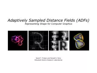
Adaptively Sampled Distance Fields (ADFs) Representing Shape for Computer Graphics
Adaptively Sampled Distance Fields (ADFs) Representing Shape for Computer Graphics. Sarah F. Frisken and Ronald N. Perry Mitsubishi Electric Research Laboratories. Outline. Overview of ADFs definition advantages instantiations Algorithms for octree-based ADFs

Adaptively Sampled Distance Fields (ADFs) Representing Shape for Computer Graphics
E N D
Presentation Transcript
Adaptively Sampled Distance Fields (ADFs)Representing Shape for Computer Graphics Sarah F. Frisken and Ronald N. Perry Mitsubishi Electric Research Laboratories
Outline • Overview of ADFs • definition • advantages • instantiations • Algorithms for octree-based ADFs • specifics of octree-based ADFs • generating, rendering, and triangulating ADFs • Applications • sculpting, scanning, meshing, modeling, machining ...
Distance Fields • A distance field is a scalar field that • specifies the distance to a shape ... • where the distance may be signed to distinguish between the inside and outside of the shape • Distance • can be defined very generally (e.g., non-Euclidean) • minimum Euclidean distance is used for most of this presentation (with the exception of the volumetric molecules)
Distance Fields -130 -95 -62 -45 -31 -46 -57 -86 -129 -90 -90 -49 -217 2516-3 -43 -90 -71 -5 30 -4 -38 -32 -3 -46 12 1 -50 -93 -3 -65 20 2D shape with sampled distances to the surface Regularly sampled distance values 2D distance field
2D Distance Field R shape Distance field of R
2D Distance Field 3D visualization of distance field of R
Shape • By shape we mean more than just the 3D geometry of physical objects. Shape can have arbitrary dimension and be derived from simulated or measured data. Color printer Color gamut
Conceptual Advantages of Distance Fields • Represent more than the surface • object interior and the space in which the object sits • Gains in efficiency and quality because • distance fields vary “smoothly” • are defined throughout space • Gradient of the distance field yields • surface normal for points on the surface • direction to closest surface point for points off the surface
Practical Advantages of Distance Fields • Smooth surface reconstruction • continuous reconstruction of a smooth field • Trivial inside/outside and proximity testing • using sign and magnitude of the distance field • Fast and simple Boolean operations • intersection: dist(AB) = min(dist(A), dist(B)) • union: dist(AB) = max(dist(A), dist(B)) • Fast and simple surface offsetting • offset by d: dist(Aoffset) = dist(A) + d • Enables geometric queries such as closest point • using gradient and magnitude of the distance field
Sampled Distance Fields • Similar to sampled images, insufficient sampling of distance fields results in aliasing • Because fine detail requires dense sampling, excessive memory is required with regularly sampled distance fields when any fine detail is present
Adaptively Sampled Distance Fields • Detail-directed sampling • high sampling rates only where needed • Spatial data structure • fast localization for efficient processing • ADFs consist of • adaptively sampled distance values … • organized in a spatial data structure … • with a method for reconstructing the distance field from the sampled distance values
ADF Instantiations • Spatial data structures • octrees • wavelets • multi-resolution tetrahedral meshes … • Reconstruction functions • trilinear interpolation • B-spline wavelet synthesis • barycentric interpolation ...
Multi-resolution Triangulation2D Spatial Data Structures - An Example
A Gallery of Examples - A Carved Vase Illustrates smooth surface reconstruction, fine carving, and representation of algebraic complexity
A Gallery of Examples - A Carved Slab Illustrates sharp corners and precise cuts
A Gallery of Examples - A Volume Rendered Molecule Illustrates volume rendering of ADFs, semi-transparency, thick surfaces, and distance-based turbulence
A Gallery of Examples - A 2D Crescent ADFs provide: • spatial hierarchy • distance field • object surface • object interior • object exterior • surface normal (gradient at surface) • direction to closest surface point (gradient off surface) ADFs consolidate the data needed to represent complex objects
ADFs - A Unifying Representation • Represent surfaces, volumes, and implicit functions • Represent sharp edges, organic surfaces, thin-membranes, and semi-transparent substances • Consolidate multiple structures for complex objects(e.g., for collision detection, LOD construction, and dynamic meshing) • Can store auxiliary data in cells or at cell vertices (e.g., color and texture)
Algorithms for Octree-based ADFs • Specifics of octree-based ADFs • Generating ADFs • Rendering ADFs • Triangulating ADFs
Octree-based ADFs • A distance value is stored for each cell corner in the octree • Distances and gradients are estimated from the stored values using trilinear reconstruction
Reconstruction A single trilinear field can represent highly curved surfaces
Comparison of 3-color Quadtrees and ADFs 23,573 cells (3-color) 1713 cells (ADF)
Bottom-up Generation Fully populate Recursively coalesce
Top-down Generation Initialize root cell Recursively subdivide
Tiled Generation • Reduced memory requirements • Better memory coherency • Reduced computation
recurSubdivToMaxLevel(cell, maxLevel, maxADFLevel) // Trivially exclude INTERIOR and EXTERIOR cells // from further subdivision pt = getCellCenter(cell) if (abs(getTileComputedDistAtPt(pt)) > getCellHalfDiagonal(cell)) // cell.type is INTERIOR or EXTERIOR setCellTypeFromCellDistValues(cell) return // Stop subdividing when error criterion is met if (cell.error < maxError) // cell.type is INTERIOR, EXTERIOR, or BOUNDARY setCellTypeFromCellDistValues(cell) return // Stop subdividing when maxLevel is reached if (cell.level >= maxLevel) // cell.type is INTERIOR, EXTERIOR, or BOUNDARY setCellTypeFromCellDistValues(cell) if (cell.level < maxADFLevel) // Tag cell as candidate for next layer setCandidateForSubdiv(cell) return // Recursively subdivide all children for (each of the cell’s 8 children) child = getNextCell(cells) initializeCell(child, cell) recurSubdivToMaxLevel(child, maxLevel, maxADFLevel) // cell.type is INTERIOR, EXTERIOR, or BOUNDARY setCellTypeFromChildrenCellTypes(cell) // Coalesce INTERIOR and EXTERIOR cells if (cell.type != BOUNDARY) coalesceCell(cell) tiledGeneration(genParams, distanceFunc) // cells: block of storage for cells // dists: block of storage for final distance values // tileVol: temporary volume for computed and // reconstructed distance values // bitFlagVol: volume of bit flags to indicate // validity of distance values in tileVol // cell: current candidate for tiled subdivision // tileDepth: L (requires (2L+1)3 volume - the L+1 // level is used to compute cell errors for level L) // maxADFLevel: preset max level of ADF (e.g., 12) maxLevel = tileDepth cell = getNextCell(cells) initializeCell(cell, NULL) (i.e., root cell) while (cell) setAllBitFlagVolInvalid(bitFlagVol) if (cell.level == maxLevel) maxLevel = min(maxADFLevel, maxLevel + tileDepth) recurSubdivToMaxLevel(cell,maxLevel,maxADFLevel) addValidDistsToDistsArray(tileVol, dists) cell = getNextCandidateForSubdiv(cells) initializeCell(cell, parent) initCellFields(cell, parent, bbox, level) for (error = 0, pt = cell, face, and edge centers) if (isBitFlagVolValidAtPt(pt)) comp = getTileComputedDistAtPt(pt) recon = getTileReconstructedDistAtPt(pt) else comp = computeDistAtPt(pt) recon = reconstructDistAtPt(cell, pt) setBitFlagVolValidAtPt(pt) error = max(error, abs(comp - recon)) setCellError(error) Tiled Generation Pseudocode
Tiled Generation - Overview • Recursively subdivide root cell to a level L • Cells at level L requiring further subdivision are appended to a list of candidate cells, C-list • These candidate cells are recursively subdivided between levels L and 2L, where new candidate cells are produced and appended to C-list • Repeat layered production of candidate cells (2L to 3L, etc.) until C-list is empty
Tiled Generation - Candidate Cells • A cell becomes a candidate for further subdivision when all of the following are true: • it is a leaf cell of level L, or 2L, or 3L, etc. • it can not be trivially determined to be an interior or exterior cell • it does not satisfy a specified error criterion • its level is below a specified maximum ADF level
Tests for Candidate Cells (1) all di have same sign (2) all || di || > ½ cell diagonal Test to trivially determine if a cell is interior or exterior 19 test points to determine cell error
Tiled Generation - Tiling • For each candidate cell, computed and reconstructed distances are produced only as needed during subdivision • These distances are stored in a tile, a regularly sampled volume • The tile resides in cache memory and its size determines L • A volume of bit flags keeps track of valid distances in the tile to ensure that distances are computed only once
Tiled Generation - Tiling • For coherency, cells and final distances are stored in two separate contiguous memory blocks • After a candidate cell has been processed, valid distances in the tile are appended to the block of final distances • Special care is taken at tile boundaries to ensure that distances are never duplicated for neighboring cells
Tiled Generation - Cache Efficiency • Tile sizes can be tuned to the CPU cache architecture • For current Pentium systems, a tile size of 163 has worked most effectively • Using a separate bit flag volume further enhances cache effectiveness and provides fast invalidation of tile distances prior to processing each candidate cell
Rendering • Ray casting • Adaptive ray casting • Point-based rendering • Triangles
Ray CastingRay-surface Intersection with a Cubic Solver • See Parker et al., ”Interactive Ray Tracing for Volume Visualization”
Ray CastingRay-surface Intersection with a Linear Solver • Assume that distances vary linearly along the ray • Determine the zero-crossing within the cell given distances at the points where the ray enters and exits the cell
Ray CastingCrackless Surface Rendering with the Linear Solver • Set the distance at the entry point of a cell equal to the distance computed for the exit point of the previous cell
Ray CastingVolume Rendering • Colors and opacities are accumulated at equally spaced samples along each ray
Adaptive Ray Casting • The image region to be rendered is divided into a hierarchy of image tiles • The subdivision of each tile is guided by a perceptually-based predicate • Pixels within image tiles of size greater than 1x1 are bilinearly interpolated to produce the image • Rays are cast into the ADF at tile corners and intersected with the surface using the linear solver
Adaptive Ray Casting • The predicate individually weights the contrast in the red, green, and blue channels and the variance in depth-from-camera across the tile • See Mitchell , SIGGRAPH’87, and Bolin and Meyer, SIGGRAPH’98 • Results in a typical 6:1 reduction in rendering time over non-adaptive ray casting
Adaptive Ray Casting Adaptively ray cast ADF Rays cast to render part of the left image
Point-based Rendering • Determine the number of points to generate in each boundary leaf cell • Compute an estimate of the object’s surface area within each boundary leaf cell areaCell and the total estimated surface area of the object,areaObject= SareaCell • Set the number of points in each cell nPtsCell proportional to areaCell / areaObject • For each boundary leaf cell in the ADF • Generate nPtsCell random points in the cell • Move each point to the object’s surface using the distance and gradient at the point
Point-based RenderingPseudocode generatePoints(adf, points, nPts, maxPtsToGen) // Estimate object’s surface area within each boundary leaf // cell and the total object’s surface area for (areaObject = 0, level = 0 to maxADFLevel) nCellsAtLevel = getNumBoundaryLeafCellsAtLevel(adf, level) areaCell[level] = sqr(cellSize(level)) areaObject += nCellsAtLevel * areaCell[level] // nPtsCell is proportional to areaCell / areaObject for (level = 0 to maxADFLevel) nPtsAtLevel[level] = maxPtsToGen * areaCell[level] / areaObject // For each boundary leaf cell, generate cell points // and move each point to the surface for (nPts = 0, cell = each boundary leaf cell of adf) nPtsCell = nPtsAtLevel[cell.level] while (nPtsCell--) pt = generateRandomPositionInCell(cell) d = reconstructDistAtPt(cell, pt) n = reconstructNormalizedGradtAtPt(cell, pt) pt += d * n n = reconstructNormalizedGradtAtPt(cell, pt) setPointAttributes(pt, n, points, nPts++)
Point-based Rendering An ADF rendered as points at two different scales
Triangle Rendering • ADFs can also be rendered by triangulating the surface and using graphics hardware to rasterize the triangles • Triangulation is fast • 200,000 triangles in 0.37 seconds, Pentium IV • 2,000 triangles in < 0.01 seconds • The triangulation produces models that are orientable and closed
Triangulation • Seed- Each boundary leaf cell of the ADF is assigned a vertex that is initially placed at the cell’s center • Join- Vertices of neighboring cells are joined to form triangles • Relax- Vertices are moved to the surface using the distance field • Improve- Vertices are moved over the surface towards their average neighbors' position to improve triangle quality
Triangulation • Vertices are joined to form triangles using the following observations • A triangle joins the vertices of 3 neighboring cells that share a common edge (hence triangles are associated with cell edges) • A triangle is associated with an edge only if that edge has a zero crossing of the distance field • The orientation of the triangle can be derived from the orientation of the edge it crosses • In order to avoid making redundant triangles, we consider 6 of the 12 possible edges for each cell
Triangulation - Surface Cracks Most triangulation algorithms for adaptive grids suffer from this type of crack; our algorithm does not As with other algorithms, this type of crack occurs very rarely but we can prevent it with a simple pre-conditioning step
Triangulation - Pre-conditioning • In 3D, the pre-conditioning step compares the number of zero-crossings of the iso-surface for each face of each boundary leaf cell to the total number of zero-crossings for faces of the cell's face-adjacent neighbors that are shared with the cell • When the number of zero-crossings are not equal for any face, the cell is subdivided using distance values from its face-adjacent neighbors until the number of zero-crossings match