Understanding Physical Database Issues and Optimization Techniques
In this lecture, we explore key physical database issues including RAID arrays for recovery and speed, and the importance of indexes for query efficiency. We discuss query optimization techniques and the use of query trees. The physical design of databases focuses on effective data storage and access, with methods to handle media failures. Additionally, the lecture provides insights into normalization processes that refine database design. For further reading, refer to Connolly and Begg's chapters on these topics to enhance your understanding of database systems.

Understanding Physical Database Issues and Optimization Techniques
E N D
Presentation Transcript
Physical DB Issues, Indexes, Query Optimisation Database Systems Lecture 13 Natasha Alechina
In This Lecture • Physical DB Issues • RAID arrays for recovery and speed • Indexes and query efficiency • Query optimisation • Query trees • For more information • Connolly and Begg chapter 21 and appendix C.5
Design so far E/R modelling helps find the requirements of a database Normalisation helps to refine a design by removing data redundancy Physical design Concerned with storing and accessing the data How to deal with media failures How to access information efficiently Physical Design
RAID - redundant array of independent (inexpensive) disks Storing information across more than one physical disk Speed - can access more than one disk Robustness - if one disk fails it is OK RAID techniques Mirroring - multiple copies of a file are stored on separate disks Striping - parts of a file are stored on each disk Different levels (RAID 0, RAID 1…) RAID Arrays
Files are split across several disks For a system with n disks, each file is split into n parts, one part stored on each disk Improves speed, but no redundancy RAID Level 0 Data Data1 Data2 Data3 Disk 1 Disk 2 Disk 3
As RAID 0 but with redundancy Files are split over multiple disks Each disk is mirrored For n disks, split files into n/2 parts, each stored on 2 disks Improves speed, has redundancy, but needs lots of disks RAID Level 1 Data Data1 Data2 Disk 1 Disk 2 Disk 3 Disk 4
We can use parity checking to reduce the number of disks Parity - for a set of data in binary form we count the number of 1s for each bit across the data If this is even the parity is 0, if odd then it is 1 1 0 1 1 0 0 1 1 0 0 1 1 0 0 1 1 1 0 1 0 1 0 0 1 0 1 1 0 1 1 1 0 0 1 0 0 0 1 1 1 Parity Checking
If one of our pieces of data is lost we can recover it Just compute it as the parity of the remaining data and our original parity information Recovery With Parity 1 0 1 1 0 0 1 1 0 0 1 1 0 0 1 1 0 1 1 0 1 1 1 0 0 1 0 0 0 1 1 1
Data is striped over disks, and a parity disk for redundancy For n disks, we split the data in n-1 parts Each part is stored on a disk The final disk stores parity information RAID Level 3 Data Data1 Data2 Data3 Parity Disk 1 Disk 2 Disk 3 Disk 4
Other RAID levels consider How to split data between disks Whether to store parity information on one disk, or spread across several How to deal with multiple disk failures Considerations with RAID systems Cost of disks Do you need speed or redundancy? How reliable are the individual disks? ‘Hot swapping’ Is the disk the weak point anyway? Other RAID Issues
Indexes are to do with ordering data The relational model says that order doesn’t matter From a practical point of view it is very important Types of indexes Primary or clustered indexes affect the order that the data is stored in a file Secondary indexes give a look-up table into the file Only one primary index, but many secondary ones Indexes
A telephone book You store people’s addresses and phone numbers Usually you have a name and want the number Sometimes you have a number and want the name Indexes A clustered index can be made on name A secondary index can be made on number Index Example
Index Example As a Table As a File Secondary Index Name Number John 925 1229 Mary 925 8923 Jane 925 8501 Mark 875 1209 Jane, 9258501 8751209 John, 9251229 9251229 Mark, 8751209 9258501 Mary, 9258923 9258923 Sometimes we look up names by number, so we index number Most of the time we look up numbers by name, so we sort the file by name Order does not really concern us here
You can only have one primary index The most frequently looked-up value is often the best choice Some DBMSs assume the primary key is the primary index, as it is usually used to refer to rows Don’t create too many indexes They can speed up queries, but they slow down inserts, updates and deletes Whenever the data is changed, the index may need to change Choosing Indexes
A product database, which we want to search by keyword Each product can have many keywords The same keyword can be associated with many products Index Example Products prodID prodName prodID keyID WordLink Keywords keyID keyWord
To search the products given a keyWord value 1. We look up the keyWord in Keywords to find its keyID 2. We look up that keyID in WordLink to find the related prodIDs 3. We look up those prodIDs in Products to find more information about them Index Example prodID prodName prodID keyID keyID keyWord
In SQL we use CREATE INDEX: CREATE INDEX <index name> ON <table> (<columns>) Example: CREATE INDEX keyIndex ON Keywords (keyWord) CREATE INDEX linkIndex ON WordLink(keyID) CREATE INDEX prodIndex ON Products (prodID) Creating Indexes
Once a database is designed and made we can query it A query language (such as SQL) is used to do this The query goes through several stages to be executed Three main stages Parsing and translation - the query is put into an internal form Optimisation - changes are made for efficiency Evaluation - the optimised query is applied to the DB Query Processing
SQL is a good language for people It is quite high level It is non-procedural Relational algebra is better for machines It can be reasoned about more easily Given an SQL statement we want to find an equivalent relational algebra expression This expression may be represented as a tree - the query tree Parsing and Translation
Product Product finds all the combinations of one tuple from each of two relations R1 R2 is equivalent to SELECT DISTINCT * FROM R1, R2 Selection Selection finds all those rows where some condition is true cond R is equivalent to SELECT DISTINCT * FROM R WHERE <cond> Some Relational Operators
Projection Projection chooses a set of attributes from a relation, removing any others A1,A2,… R is equivalent to SELECT DISTINCT A1, A2, ... FROM R Projection, selection and product are enough to express queries of the form SELECT <cols> FROM <table> WHERE <cond> Some Relational Operators
SQL statement SELECT Student.Name FROM Student, Enrolment WHERE Student.ID = Enrolment.ID AND Enrolment.Code = ‘DBS’ Relational Algebra Take the product of Student and Enrolment select tuples where the IDs are the same and the Code is DBS project over Student.Name SQL Relational Algebra
Query Tree pStudent.Name sStudent.ID = Enrolment.ID sEnrolment.Code = ‘DBS’ Student Enrolment
There are often many ways to express the same query Some of these will be more efficient than others Need to find a good version Many ways to optimise queries Changing the query tree to an equivalent but more efficient one Choosing efficient implementations of each operator Exploiting database statistics Optimisation
In our query tree before we have the steps Take the product of Student and Enrolment Then select those entries where the Enrolment.Code equals ‘DBS’ This is equivalent to selecting those Enrolment entries with Code = ‘DBS’ Then taking the product of the result of the selection operator with Student Optimisation Example
Optimised Query Tree pStudent.Name sStudent.ID = Enrolment.ID Student sEnrolment.Code = ‘DBS’ Enrolment
To see the benefit of this, consider the following statistics Nottingham has around 18,000 full time students Each student is enrolled in at about 10 modules Only 200 take DBS From these statistics we can compute the sizes of the relations produced by each operator in our query trees Optimisation Example
Original Query Tree pStudent.Name 200 200 sStudent.ID = Enrolment.ID 3,600,000 sEnrolment.Code = ‘DBS’ 3,240,000,000 18,000 180,000 Student Enrolment
Optimised Query Tree p Student.Name 200 200 sStudent.ID = Enrolment.ID 3,600,000 200 18,000 Student sEnrolment.Code = ‘DBS’ 180,000 Enrolment
The original query tree produces an intermediate result with 3,240,000,000 entries The optimised version at worst has 3,600,000 A big improvement! There is much more to optimisation In the example, the product and the second selection can be combined and implemented efficiently to avoid generating all Student-Enrolment combinations Optimisation Example
If we have an index on Student.ID we can find a student from their ID with a binary search For 18,000 students, this will take at most 15 operations For each Enrolment entry with Code ‘DBS’ we find the corresponding Student from the ID 200 x 15 = 3,000 operations to do both the product and the selection. Optimisation Example
Next Lecture • Transactions • ACID properties • The transaction manager • Recovery • System and Media Failures • Concurrency • Concurrency problems • For more information • Connolly and Begg chapter 20 • Ullman and Widom chapter 8.6