Download
1 / 83
830 likes | 965 Views
Multivariate Description. What Technique?. a) Rotate the Variable Space. Raw Data. Linear Regression. Two Regressions. Principal Components. Gulls Variables. Scree Plot. Output. > summary(gulls.pca2) Importance of components:

E N D
Output > summary(gulls.pca2) Importance of components: Comp.1 Comp.2 Comp.3 Standard deviation 1.8133342 0.52544623 0.47501980 Proportion of Variance 0.8243224 0.06921464 0.05656722 Cumulative Proportion 0.8243224 0.89353703 0.95010425 > gulls.pca2$loadings Loadings: Comp.1 Comp.2 Comp.3 Comp.4Weight -0.505 -0.343 0.285 0.739Wing -0.490 0.852 -0.143 0.116Bill -0.500 -0.381 -0.742 -0.232H.and.B -0.505 -0.107 0.589 -0.622
Linear Discriminant > gulls.lda <- lda(Sex ~ Wing + Weight + H.and.B + Bill, gulls) lda(Sex ~ Wing + Weight + H.and.B + Bill, data = gulls) Prior probabilities of groups: 0 1 0.5801105 0.4198895 Group means: Wing Weight H.and.B Bill0 410.0381 871.7619 115.1143 17.625241 430.6118 1054.3092 125.9474 19.50789 Coefficients of linear discriminants: LD1Wing 0.045512619Weight 0.001887236H.and.B 0.138127194Bill 0.444847743
Uses of Distances Distance/Dissimilarity can be used to:- • Explore dimensionality in data(using PCO) • As a basis for clustering/classification
Species and Sites as Weighted Averages of each other SITES 1 1 1111 1 2111 SPP. 23466185750198304927 Bel per 3.2....2..2..22..... Jun buf .3..........4..…42.. Jun art ...3..4..3..4..4.... Air pra ........2........3.. Ele pal ...8..4..5.....44... Rum ace ....6..5....2..…23.. Vic lat ..........12.1...... Bra rut ..246.22.4242624.342 Ran fla .2.2..2..2.....42... Hyp rad ........2..2.....5.. Leo aut 522.3.33223525222623 Pot pal .........2......2... Poa pra 424.34421.44435.…4.. Cal cus ...3...........34... Tri pra ....5..2........…2.. Tri rep 521.5.22.163322.6232 Ant odo ....3..44.4......4.2 Sal rep .............3.5.3.. Ach mil 3...21.22.4.....…2.. Poa tri 79524246..4.5.6…45.. Ely rep 4.4..4.4....6.4..... Sag pro .25...2....22....34. Pla lan ....5..52.33.3..…5.. Agr sto .587..4..4..3.454.4. Lol per 5.5.6742..67226.…6.. Alo gen 2524..5.....3.7...8. Bro hor 4.3....2..4.....…2..
Site A B C D E F SpeciesPrunus serotina 6 3 4 6 5 1 Tilia americana2 0 7 0 6 6Acer saccharum0 0 8 0 4 9 Quercus velutina0 8 0 8 0 0 Juglans nigra3 2 3 0 6 0 Reciprocal Averaging - unimodal
Site A B C D E F Species ScoreSpecies Iteration 1Prunus serotina 6 3 4 6 5 1 1.00Tilia americana2 0 7 0 6 60.63Acer saccharum0 0 8 0 4 9 0.63Quercus velutina0 8 0 8 0 0 0.18Juglans nigra3 2 3 0 6 00.00 Iteration11.00 0.00 0.86 0.60 0.62 0.99SiteScore Reciprocal Averaging - unimodal
Site A B C D E F Species ScoreSpecies Iteration 12Prunus serotina 6 3 4 6 5 1 1.00 0.68Tilia americana2 0 7 0 6 6 0.63 0.84Acer saccharum0 0 8 0 4 9 0.63 0.87Quercus velutina0 8 0 8 0 0 0.18 0.30Juglans nigra3 2 3 0 6 0 0.00 0.67 Iteration 1 1.00 0.00 0.86 0.60 0.62 0.99Site20.65 0.00 0.88 0.05 0.78 1.00Score Reciprocal Averaging - unimodal
Site A B C D E F Species ScoreSpecies Iteration 1 23Prunus serotina 6 3 4 6 5 1 1.00 0.68 0.50Tilia americana2 0 7 0 6 6 0.63 0.84 0.86Acer saccharum0 0 8 0 4 9 0.63 0.87 0.91Quercus velutina0 8 0 8 0 0 0.18 0.30 0.02Juglans nigra3 2 3 0 6 0 0.00 0.67 0.66 Iteration 1 1.00 0.00 0.86 0.60 0.62 0.99Site 2 0.65 0.00 0.88 0.05 0.78 1.00Score30.60 0.01 0.87 0.00 0.78 1.00 Reciprocal Averaging - unimodal
Site A B C D E F Species ScoreSpecies Iteration 1 2 3 9Prunus serotina 6 3 4 6 5 1 1.00 0.68 0.50 0.48Tilia americana2 0 7 0 6 6 0.63 0.84 0.86 0.85Acer saccharum0 0 8 0 4 9 0.63 0.87 0.91 0.91Quercus velutina0 8 0 8 0 0 0.18 0.30 0.02 0.00Juglans nigra3 2 3 0 6 0 0.00 0.67 0.66 0.65 Iteration 1 1.00 0.00 0.86 0.60 0.62 0.99Site 2 0.65 0.00 0.88 0.05 0.78 1.00Score 3 0.60 0.01 0.87 0.00 0.78 1.0090.59 0.01 0.87 0.00 0.78 1.00 Reciprocal Averaging - unimodal
Site A C E B D F Species Species ScoreQuercus velutina8 8 0 0 0 0 0.004Prunus serotina6 3 6 5 4 10.477Juglans nigra0 2 3 6 3 0 0.647Tilia americana0 0 2 6 7 6 0.845Acer saccharum0 0 0 4 8 9 0.909 Site Score0.000 0.008 0.589 0.778 0.872 1.000 Reordered Sites and Species
Managing Dimensionality (but not acronyms)PCA, CA, RDA, CCA, MDS, NMDS, DCA, DCCA, pRDA, pCCA
Type of Data Matrix species attributes desert macroph inverts uses species sites attributes attributes watervar rain gulls individuals sites
Models of Species Response There are (at least) two models:- • Linear - species increase or decrease along the environmental gradient • Unimodal - species rise to a peak somewhere along the environmental gradient and then fall again
Alpha and Beta Diversity • alpha diversity is the diversity of a community (either measured in terms of a diversity index or species richness) • beta diversity (also known as ‘species turnover’ or ‘differentiation diversity’) is the rate of change in species composition from one community to another along gradients; gamma diversity is the diversity of a region or a landscape.
Indirect Gradient Analysis • Environmental gradients are inferred from species data alone • Three methods: • Principal Component Analysis - linear model • Correspondence Analysis - unimodal model • Detrended CA - modified unimodal model
PCA gradient - site/species biplot standard biodynamic& hobby nature
The Arch Effect • What is it? • Why does it happen? • What should we do about it?