Output and Expenditure in the Short Run

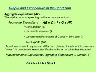
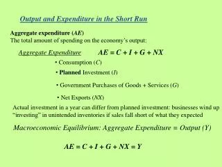
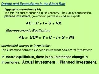
1. Output and Expenditure in the Short Run Aggregate expenditure (AE)The total amount of spending on the economy’s output: AE = C + I + G + NX Aggregate Expenditure • Consumption (C) • Planned Investment (I) • Government Purchases of Goods + Services (G) • Net Exports (NX) Actual investment in a year can differ from planned investment: businesses wind up “investing” in unintended inventories if sales fall short of what they expected Macroeconomic Equilibrium: Aggregate Expenditure = Output (Y) AE = C + I + G + NX = Y

2. The Aggregate Expenditure Model Adjustments to Macroeconomic Equilibrium Actual investment in a year can differ from planned investment: businesses “invest” in unintended inventories if sales fall short of what they expected

3. Components of Real Aggregate Expenditure, 2010

4. Consumption Real Consumption Consumption follows a smooth, upward trend, interrupted only infrequently by brief recessions.

5. The most important variables that determine the level of C: • Current disposable income • Household wealth: Assets minus liabilities Including equity in owner occupied houses?

6. Do Changes in Housing Wealth Affect Consumption Spending? Housing wealth equals the market value of houses minus the value of loans people have taken out to pay for the houses = Homeowner Equity The figure shows the S&P/Case-Shiller index of housing prices, which represents changes in the prices of single-family homes. Because many macroeconomic variables move together, economists sometimes have difficulty determining whether movements in one are causing movements in another.

7. The most important variables that determine the level of C: • • Current disposable income • • Household wealth: Assets minus liabilities • Including equity in owner occupied houses? • • Expected future income • People try to keep their consumption fairly steady from year-to-year •  tie consumption to “permanent income” and save for a rainy day • • The price level • Higher price level reduces real value of monetary wealth • • The interest rate • High interest rate discourages spending on credit/encourages saving • New, gotta-have styles and products

8. The most important determinant of consumption is: • Current disposable income • Household wealth. • Expected future income. • The price level and the interest rate.

9. The Consumption Function • The Relationship between Consumption and Income, 1960–2010 • The Slope of the Consumption Function is the Marginal Propensity to Consume • MPC = Change in Consumption in Response to a Change in Disposable Income • MPC = ΔConsumption/ΔDisposable Income = ΔC/ΔYD • When disposable income changes, ΔC= MPC x ΔYD

10. For a textbook economy: The Relationship between Consumption and National Income when net taxes are constant  ΔYD = ΔNI

11. Which of the following is correct? • Disposable income is equal to national income plus government transfer payments minus taxes. • Taxes minus Government transfer payments equal net taxes. • Disposable income = National income – Net taxes. • All of the above.

12. Income, Consumption, and Saving National income = Consumption + Saving + Net Taxes Y = C + S + T Change in NI = Change in consumption + Change in saving + Change in taxes If taxes are always a constant amount, ΔT = 0 ΔY = ΔC + ΔS 1 = MPC + MPS

13. Calculating the Marginal Propensity to Consume and the Marginal Propensity to Save Fill in the blanks in the following table. For simplicity, assume that taxes are zero.

14. Calculating the Marginal Propensity to Consume and the Marginal Propensity to Save Fill in the blanks in the following table. For simplicity, assume that taxes are zero. Fill in the table. For example, to calculate the value of the MPC in the second row, we have: To calculate the value of the MPS in the second row, we have:

15. Calculating the Marginal Propensity to Consume and the Marginal Propensity to Save Fill in the blanks in the following table. For simplicity, assume that taxes are zero. Show that the MPC plus the MPS equals 1. Show that the MPC plus the MPS equals 1. At every level of national income, the MPC is 0.6 and the MPS is 0.4. Therefore, the MPC plus the MPS is always equal to 1.

16. If the marginal propensity to consume (MPC) is 0.9, how much additional consumption will result from an increase of $80 billion of disposable income? • $88.89 billion. • $800 billion. • $72 billion. • None of the above.

17. Planned Investment Real Investment Investment is subject to larger changes than is consumption. Investment declined significantly during the recessions of 1980, 1981–1982, 1990–1991, 2001, and 2007–2009. Note: The values are quarterly data, seasonally adjusted at an annual rate.

18. The most important variables that determine the level of investment: • • Expectations of future profitability • Waves of optimism and pessimism • • Major technology changes: new products & processes • The interest rate • • Taxes • • Cash flow  Retained earnings for financing investment • Current capacity utilization

19. The behavior of consumption and investment over time can be described as follows: • Investment follows a smooth, upward trend, but consumption is highly volatile. • Consumption follows a smooth, upward trend, but investment is subject to significant fluctuations. • Both consumption and investment fluctuate significantly over time. • Neither consumption nor investment fluctuate significantly over time.

20. Government Purchases (including State and Local) = G Real Government Purchases Government purchases grew steadily for most of the 1979–2011 period, with the exception of the early 1990s, when concern about the federal budget deficit caused real government purchases to fall for three years, beginning in 1992and in recent recession when State and Local expenditures declined.

21. Real Net Exports Net exports were negative in most years between 1979 and 2011. Net exports have usually increased when the U.S. economy is in recession and decreased when the U.S. economy is expanding, although they fell during most of the 2001 recession. Note: The values are quarterly data, seasonally adjusted at an annual rate.

22. Net Exports (NX) The most important variables that determine the level of net exports: • The price level in the United States relative to the price levels in other countries • The growth rate of GDP in the United States relative to the growth rates of GDP in other countries • The exchange rate between the dollar and other currencies

23. If inflation in the United States is lower than inflation in other countries, then U.S. exports ________ and U.S. imports ________, which _________ net exports. • increase; increase; decreases • increase; decrease; increases • decrease; increase; increases • decrease; increase; decreases

24. Graphing Macroeconomic Equilibrium The Relationship between Planned Aggregate Expenditure and GDP on a 45°-Line Diagram

25. Graphing Macroeconomic Equilibrium

26. Graphing Macroeconomic Equilibrium

27. Showing a Recession on the 45°-Line Diagram

28. Macroeconomic Equilibrium

29. The Multiplier Effect

30. Learning Objective 11.4 The Multiplier Effect Autonomous expenditure An expenditure that does not depend on the level of GDP. Multiplier The increase in equilibrium real GDP in response to increase in autonomous expenditure, e.g. Expenditure multiplier = ΔY/ΔI Multiplier effect The process by which an increase in autonomous expenditure leads to a larger increase in real GDP: ΔY = ΔI + ΔC = Change in autonomous spending that sparks an expansion + Change in consumption spending induced by increasing output and income.

31. The Multiplier Effect in Action

32. MakingtheConnection • The Multiplier in Reverse: The Great Depression of the 1930s The multiplier effect contributed to the very high levels of unemployment during the Great Depression.

33. The Multiplier Effect A Formula for the Multiplier Y = C + I + G + NX C depends on YD: C = c0 + MPC x YD = c0 + MPC x (Y – T) c0, I, G, T, and NX are autonomous—they do not depend on Y Y = c0 + MPC x Y – MPC x T + I + G + NX (1 – MPC) x Y = c0 + I + G – MPC x T + NX Y = [1/(1 – MPC)] x [c0 + I + G – MPC x T + NX]

34. Find equilibrium GDP using the following macroeconomic model: • C = 1000 + 0.75Y Consumption function • I = 500 Investment function • G = 600 Government spending function • NX = −300 Net export function • Y = C + I + G + NX Equilibrium condition • 800 • 1800 • 2400 • 7200

35. Summarizing the Multiplier Effect 1The multiplier effect occurs both when autonomous expenditure increases and when it decreases. 2The multiplier effect makes the economy more sensitive to changes in autonomous expenditure than it would otherwise be. 3The larger the MPC, the larger the value of the multiplier. 4 The formula for the multiplier, 1/(1 − MPC), is oversimplified because it ignores some real-world complications, such as the effect that an increasing GDP can have on taxes, imports, prices and interest rates.

36. Using the Multiplier Formula Use the information in the table to answer the following questions: a. What is the equilibrium level of real GDP? b. What is the MPC? c. If government purchases increase by $200 billion, what will be the new equilibrium level of real GDP? Use the multiplier formula to determine your answer.

37. Using the Multiplier Formula Use the information in the table to answer the following questions: Determine equilibrium real GDP. We can find macroeconomic equilibrium by calculating the level of planned aggregate expenditure for each level of real GDP. We can see that macroeconomic equilibrium will occur when real GDP equals $10,000 billion. Calculate the MPC. In this case:

38. Using the Multiplier Formula Use the multiplier formula to calculate the new equilibrium level of real GDP. We could find the new level of equilibrium real GDP by constructing a new table with government purchases increased from $1,000 billion to $1,200 billion. But the multiplier allows us to calculate the answer directly. In this case: So: Change in equilibrium real GDP = Change in autonomous expenditure × 5 Or: Change in equilibrium real GDP = $200 billion × 5 = $1,000 billion Therefore: New level of equilibrium GDP = $10,000 billion + $1,000 billion = $11,000 billion

39. The Paradox of Thrift In discussing the aggregate expenditure model, John Maynard Keynes argued that if many households decide at the same time to increase their saving and reduce their spending, they may make themselves worse off by causing aggregate expenditure to fall, thereby pushing the economy into a recession. The lower incomes in the recession might mean that total saving does not increase, despite the attempts by many individuals to increase their own saving. Keynes referred to this outcome as the paradox of thrift because what appears to be something favorable to the long-run performanceof the economy might be counterproductive in the short run.

40. Aggregate Demand: The Relation Between Price and Aggregate Expenditure • Increases in the price level cause aggregate expenditure to fall, and decreases in the price level cause aggregate expenditure to rise. • There are three main reasons for this inverse relationship between changes in the price level and changes in aggregate expenditure: • A rising price level decreases Consumption by decreasing the real value of household wealth • International competition: If the price level in the United States rises relative to the price levels in other countries, U.S. exports will become relatively more expensive, and foreign imports will become relatively less expensive, causing Net Exports to fall. • Interest rate effect: When prices rise, firms and households need more money to finance buying and selling. If the central bank does not increase the money supply, the result will be an increase in the interest rate, which causes Investment spending to fall. Rising interest rates may also lead to dollar appreciation: U.S. exports will become relatively more expensive, and foreign imports will become relatively less expensive, causing Net Exports to fall yet more.

41. The Aggregate Demand Curve The Effect of a Change in the Price Level on Real GDP

42. Aggregate demand curve A curve that shows the relationship between the price level and the level of planned aggregate expenditure, holding constant all other factors that affect aggregate expenditure.

43. K e y T e r m s Aggregate demand curve Aggregate expenditure (AE) Aggregate expenditure model Autonomous expenditure Cash flow Consumption function Inventories Marginal propensity to consume (MPC) Marginal propensity to save (MPS) Multiplier Multiplier effect

44. Appendix 1 Consumption function 2 Planned investment function 3 Government spending function 4 Net export function 5 Equilibrium condition • The Algebra of Macroeconomic Equilibrium

45. Appendix The letters with bars over them represent fixed, or autonomous, values. So, represents autonomous consumption, which had a value of 1,000 in our original example. Now, solving for equilibrium, we get: Or,Or,Or, • The Algebra of Macroeconomic Equilibrium

46. Appendix Remember that is the multiplier. Therefore an alternative expression for equilibrium GDP is: • The Algebra of Macroeconomic Equilibrium Equilibrium GDP = Autonomous expenditure x Multiplier