Download
1 / 63
690 likes | 959 Views
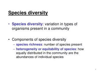
Species diversity. Concept of diversity. Informally … variety Wallace’s traveler

E N D
Concept of diversity • Informally … variety • Wallace’s traveler • A traveler in Amazonia encounters a species of tree (1 individual); If he looks for another member of that same species he will seek it for a long time, encountering many other species before he finds another. This is true for most if not all the tree species in Amazonia.
Concept of diversity • In contrast … cattail marsh • for one species, number of encounters between successive encounters with the same species will be small (often 0) • Intuitively, Amazon forest is more diverse than the cattail marsh
Diversity • Equivalent to • probability of interspecific encounter • average rarity • What determines these? • 1) number of species (S ) … species richness • 2) evenness, or equitability, or relative abundances (E )
Kinds of diversity • a diversity: variety of species within one community • b diversity: extent of replacement of species with changes in environment from place to place • g diversity: combination of a and b diversity
Numbers, measurements, etc. • S = number of species • N = number of individuals • ni= number of individuals of species i • i= 1, 2, 3, … , S • Si=1ni= N • pi= ni/ N = relative abundance of species i
Sn Sn ni ni Sn Sn ni ni Graphical representation of E Sn= number of species with abundance ni,
Quantifying evenness • (observed diversity / maximal diversity) for a given S • Calculate some measure of overall diversity (D) • Hold S constant and set relative abundances of all species to 1/S • Calculate Dmax= maximal diversity • E = D / Dmax
Diversity indices • Single number combining species number and evenness • >60 different formulas • differ in relative weight given to evenness or species number
Three examples • S - 1 = D 1 • gives 0 weight to evenness • Shannon-Weiner: - Si=1piln(pi) = D2 • intermediate weight to evenness • Simpson’s: 1 - Si pi2 = D3 • gives major weight to evenness • Used to compare communities
Different comparisons • Indices do not measure a single quantity • Diversity indices combine 2 inherently different quantities • Weights chosen are arbitrary • Indices are related in a complex way
R(pi) pi General form of diversity indices • Average rarity = diversity • a community composed of many rare species is diverse • Rarity ( R (pi)) is a decreasing function of relative abundance (pi)
S S Sni(R (pi)) Spi(R (pi)) = N General form of diversity indices Average rarity = = D [A diversity index]
encounters: • i … j … k … m… j … x … z … i • y = 6 What is R ( pi ) ? Rarity indicated by number of encounters y with other species that occur between encounters of a given species y is amenable to analysis via probability theory
From y to R ( pi) • In general, probability theory yields the general function: R ( pi ) = (1 - pib) / b • where b is a constant chosen by investigator
D = average rarity(a general diversity index) • D = Spi R( pi ) = Spi [ (1 - pib) / b ] • constant b that is chosen determines which of the diversity indices (S-1, Shannon, Simpson) results • as b increases, greater weight is given to evenness
Diversity indices • Shows that they are related • Differ in R( pi) • Does not solve the problem… which weighting is correct • Solution: don’t bother with diversity indices • implies that diversity as a single thing doesn’t exist
Quantifying diversity • Report S • in a sample S depends on N • to compare samples of different sizes use rarefaction • Report E • many measures depend on S • choose those least dependent on S
Rarefaction • two samples of different N • lower N, lower S in the sample, regardless of S in the community itself • Rarefaction … estimating expected number of species in a sample of size n : • E (S )n
E (S)n = s (N - ni)! N ! S 1 - n! (N - ni - n)! n! (N - n) ! Rarefaction N = number of individuals in entire sample n = number of individuals in the subsample ni= number of individuals in species i
Example • Communities A and B • differ in S and N in sample • How many species are expected in B if only 16 individuals were sampled?
Example • N = 62, n = 16, ni = {10, 20, 10, 20, 2} • E (S )n = 0.962 + 0.999 + 0.962 + 0.999 + 0.453 • = 4.376 • i.e., 4 or 5 species from community B • Even with rarefaction, community B has greater species richness
When to use rarefaction • If NA and NB are close, rarefaction makes little difference • Rule of thumb: if NA / NB > 10 or < 0.1 then use rarefaction
Evenness • Quantification should be independent of S • Smith & Wilson 1996 tested 14 indices • Most, including common ones, fail • note: Morin p. 18 J = H’ / Hmax • = [-Spi ln pi ]/[ln S ] • one of the worst for independence of S
Evenness • example: Modified Hill’s Ratio • claimed to be less dependent on S than most • E = {(1 / Spi2) - 1} / {exp(-Spi ln pi ) - 1} • dominance by 1 species … E = 0 • maximal evennesss … E = 1 • Smith & Wilson show it is independent of S only for S > 10
Evenness • among those that are independent of S: E1/D = 1 / (SSpi2) & Evar = 1 – (2/p){arctan[VAR(ln(ni))]} = 1 – (2/p){arctan S[ln(ni) – Sln(ni)/S]2 / S} • seem to be good choices
Evenness • E1/D… simple • Evar … derived from variance, hence derived from the conceptual basis of evenness
b diversity • Extent of replacement of species from place to place • May be equated to dissimilarity between locations • If all locations have identical species list, b diversity is 0
b diversity • Whittaker defined b diversity as; • b=g/a • Where g is regional diveristy • And a is local diversity • However • Debate about additive vs. multiplicative relationship of a b g • g=ab vs. g=a+b
Quantifying b diversity • Inversely related to similarity • Two samples • a=species unique to community A • b=species unique to community B • c=species shared • Jaccard’s similarity J = c/(a+b+c) • Sørensen’s similarity Ø = 2c/(a+c+b+c) • 1-similarity = distance or turnover
Quantifying b diversity • Whittaker’s index • b = (a+b+c)/{[a+c+b+c]/2} – 1 • = (Stotal /S)-1 • Works with >2 samples. • NOTE: none of these weight species by abundances • (i.e., none incorporate evenness)
b diversity • Thorough mathematical treatments of b diversity • Tuomista 2010 a, b • Jost 2007 • But the more interesting question is why do we care about b diversity? • component of biodiversity that is at least in part independent of a diversity • Relationships of biotic variables to a b g are not consistent
How is S related to primary productivity? • Small scale • fertilize plots - plant diversity declines • Tilman 1996 (Fig. 2c) • Lakes • Eutrophication - diversity declines
species productivity Unimodal diversity-productivity gradients
species productivity Monotonic diversity-productivity gradients
species productivity Unimodal can look like monotonic
Why should diversity decline with productivity? • High productivity reduced spatial heterogeneity in resources • Spatial heterogeneity fosters diversity • reduces competitive exclusion • variance in resource ratio hypothesis (VRR) • each species does best on a particular ratio of resources • e.g., plants and soil nutrients
Spatial heterogeneity of resources • Tilman’s fertilizer experiment • add N to soil • changes resource ratio • as N goes up greatly, ratio of N to other nutrients gets larger and more constant • Varying resource ratios do foster coexistence among plants • other taxa?
VRR Hypothesis • Assumes • species occur in patches • competition is local • resource competition • Generality? • Rodents? • Benthic invertebrates? • Tropical mammals?
Scale • Local plots Continental areas • relationships of diversity to productivity differ • Chase & Leibold 2002; Gross et al 2000 • Unimodal patterns at local scale • Monotonic* patterns at regional scales • Implication: b diversity increases with productivity * Increasing
Scale Same mechanism at all scales? VRR works best at local plot scale Applicability at larger scales unknown Does natural variation in productivity affect species the same way as experimental manipulation?
Alternative interpretations (Abrams 1995) • Challenges interpretation of monotonic patterns as artefacts of inadequate sampling • Questions the assumption that unimodal patterns must be due to competition • need for experimental data on competition • experimental test of VRR • Alternative hypotheses predict monotonic relationships
How is S related to stability? • What is stability? • Mathematically, a stable equilibrium… • for variables i = 1 to n: dXi / dt = 0 • if the system is perturbed away from equilibrium (X1, X2, … Xn)* it returns • GLOBAL STABILITY: returns from any perturbation • LOCAL STABILITY: returns from a limited set of perturbations
Ecological stability has multiple facets • Constancy: lack of change in a variable • Resiliency: continued functioning despite change • Recovery: return to original state • elasticity greater if return in more rapid • Inertia: resistance to change via perturbation • Persistence: survival of the system despite changes (no extinctions)
Ecological stability • Populations may be stable in number of individuals • Communities may be stable in: • species number • total biomass • Gross primary productivity • species abundance patterns