Emagram Stüve diagram

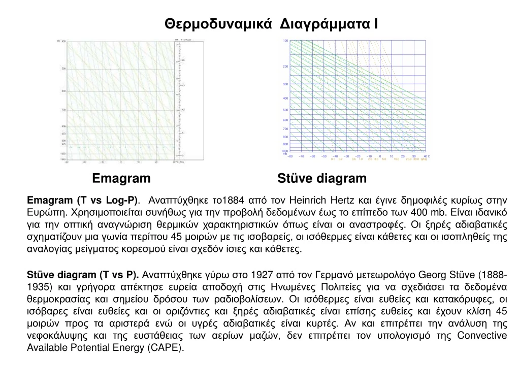
1. Θερμοδυναμικά Διαγράμματα Ι Emagram                                   Stüve diagram Emagram (T vs Log-P).  Αναπτύχθηκε το1884 από τον Heinrich Hertz και έγινε δημοφιλές κυρίως στην Ευρώπη. Χρησιμοποιείται συνήθως για την προβολή δεδομένων έως το επίπεδο των 400 mb. Είναι ιδανικό για την οπτική αναγνώριση θερμικών χαρακτηριστικών όπως είναι οι αναστροφές. Οι ξηρές αδιαβατικές σχηματίζουν μια γωνία περίπου 45 μοιρών με τις ισοβαρείς, οι ισόθερμες είναι κάθετες και οι ισοπληθείς της αναλογίας μείγματος κορεσμού είναι σχεδόν ίσιες και κάθετες. Stüve diagram (T vs P).Αναπτύχθηκε γύρω στο 1927 από τον Γερμανό μετεωρολόγο Georg Stüve (1888-1935) και γρήγορα απέκτησε ευρεία αποδοχή στις Ηνωμένες Πολιτείες για να σχεδιάσει τα δεδομένα θερμοκρασίας και σημείου δρόσου των ραδιοβολίσεων. Οι ισόθερμες είναι ευθείες και κατακόρυφες, οι ισόβαρες είναι ευθείες και οι οριζόντιες και ξηρές αδιαβατικές είναι επίσης ευθείες και έχουν κλίση 45 μοιρών προς τα αριστερά ενώ οι υγρές αδιαβατικές είναι κυρτές. Αν και επιτρέπει την ανάλυση της νεφοκάλυψης και της ευστάθειας των αερίων μαζών, δεν επιτρέπει τον υπολογισμό της Convective Available Potential Energy (CAPE).

2. Θερμοδυναμικά Διαγράμματα ΙΙ Skew-T Log-P      Tephigram Skew-T Log-P.  Αναπτύχθηκε το 1947 από τον N. Herlofson και έγινε το πιο δημοφιλές διάγραμμα στις ΗΠΑ. Είναι το καλύτερο για να εμφανίζονται δεδομένα μέχρι το επίπεδο των 100 mb. Η κατασκευή του διαγράμματος είναι παρόμοια με εκείνη του Emagram (βλέπε παρακάτω), αλλά οι γραμμές θερμοκρασίας γέρνουν περίπου 45 μοίρες προς τα δεξιά, η οποία προσανατολίζει τα δεδομένα ραδιοβόλησης σε μια κατακόρυφη κατακόρυφη εικόνα. Tephigram (T- phi -gram). Αναπτύχθηκε από το Napier Shaw το 1915 και έγινε δημοφιλές στην Αγγλία. Οι αλγόριθμοι κατασκευής του είναι πιο πολύπλοκοι από τα παραπάνω διαγράμματα και επομένως χρησιμοποιούνται σπάνια από προγράμματα αυτοματοποιημένων προγραμμάτων σχεδίασης. Στο Τεφίγραμμα οι ισοθερμίες είναι ευθείες και έχουν κλίση 45 μοιρών προς τα δεξιά ενώ οι ισοβάθρες είναι οριζόντιες και έχουν ελαφρά καμπύλη. Τα ξηρά αδιαβατικά είναι επίσης ευθεία και έχουν κλίση 45 μοιρών προς τα αριστερά ενώ οι υγρές αδιαβλαβείς είναι καμπύλες.

3. Τεφίγραμμα • Επιτρέπει την ανάλυση συνθηκών ευστάθειας από μία ραδιοβόλισησε διάφορα στρώματα • Επιτρέπει υπολογισμούς που περιλαμβάνουν την υγρασία σε διάφορα στρώματα • Επιτρέπει τον προσδιορισμό διάφορων αέριων μαζών • Βοηθά στο αναγνωρισμό νεφών και διάφορων φυσικών διεργασιών • Επιτρέπει υπολογισμούς και συγκρίσεις της Convective Available Potential Energy (CAPE) καθώς έχει την ιδιότητα οι περιοχές που περιέχονται στις καμπύλες να έχουν ίσες ενέργειες για ίσα εμβαδά.

4. Βασική ιδέα • Θερμοκρασία στονάξονα x και εντροπία στον άξονα y • dS = cpdlnθοπότετο διάγραμμα είναι θερμοκρασία σε σχέση με lnθ

5. Προσθέτουμε τη πίεση Οι κυρτές γραμμές είναι ισοπληθείς πίεσης σε mb.

6. Περιστροφή και σχεδιασμός Το διάγραμμα περιστρέφεται κατά 45°έτσι ώστε οι ισοβαρείς να είναι σχεδόν οριζόντιες Οι μετρήσεις θερμοκρασίας (T) και θερμοκρασίας του σημείου δρόσου (Td) σημειώνονται στο διάγραμμα.

7. Προσθέτουμε πληροφορία σχετικά με την υγρασία • Η θερμοκρασία του σημείου δρόσου είναι ένα μέτρο της υγρασίας στην ατμόσφαιρα. Το τεφίγραμμα μπορεί να χρησιμοποιηθεί για να μετατρέψει (TD,T) σε αναλογία μείγματος υδρατμών. • Ισοπληθείς της αναλογίας μείγματος των υδρατμών προσθέτονται στο Τεφίγραμμα ως διακεκομμένες γραμμές (μονάδες g/kg). • Κυρτές γραμμές επίσης προσθέτονται και δηλώνουν τις υγρές κορεσμένες αδιαβατικές καμπύλες.

9. Τεφίγραμμα Υγρές κορεσμένες αδιαβατικές Αναλογία μείγματος υδρατμών

10. Τεφίγραμμα

11. Τεφίγραμμα

12. TεφίγραμμαΆσκηση 1 1. Προσθέτουμε τη θερμοκρασία Τ

13. TεφίγραμμαΆσκηση 1 1. Προσθέτουμε τη θερμοκρασία Τ

14. TεφίγραμμαΆσκηση 1 2.Προσθέτουμε τη θερμοκρασία του σημείου δρόσου Td

15. TεφίγραμμαΆσκηση 1 2. Προσθέτουμε τη θερμοκρασία του σημείου δρόσου Td

16. TεφίγραμμαΆσκηση 1 Δυνητική θερμοκρασία στα 800 hPa, Θ=291K Στα 1000 hPa Θ=?

17. TεφίγραμμαΆσκηση 1 π.χ. στα 1000 hPa RH=r/rs =5/7.7=65% στα 800 hPa RH= ? π.χ. στα 1000 hPa r= 5 g/kg στα 800 hPa r= ? π.χ. στα 1000 hPa rs= 7.7 g/kg στα 800 hPa rs= ? 3. Προσδιορισμός r, rs και RH

18. TεφίγραμμαΆσκηση 1 π.χ.για στα 1000 hPa προεκτείνω την ισόθερμη στα 622 hPa e= 8.2 hPa για τα 800 hPae= ? π.χ. στα 1000 hPa RH=e/es =8.2/12.6=65% στα 800 hPa RH= ? r=0.622 e/P rs=0.622es/P π.χ.για στα 1000 hPa προεκτείνω την ισόθερμη στα 622 hPa es= 12.6 hPa για τα 800 hPaes= ? 4. Προσδιορισμός e και es

19. TεφίγραμμαΆσκηση 1 Πάχος περίπου 1 km Πάχος οριακού στρώματος?

20. TεφίγραμμαΆσκηση 1 π.χ. στα 1000 hPa θ=285 Κ στα 950 hPa θ= 285Κ στα 900 hPa θ= 285Κ π.χ. στα 1000 hPa r= 5 g/kg στα 950 hPa r= 5 g/kg στα 900 hPa r= 5 g/kg Είναι το οριακό στρώμα καλά αναμεμειγμένο?

21. TεφίγραμμαΆσκηση 1 LCL :910 hPa 5. Προσδιορισμός LCL (επίπεδο συμπυκνωσης από εξαναγκασμένη άνοδο)

22. TεφίγραμμαΆσκηση 1 CCL :810 hPa Tc :18oC 6. Προσδιορισμός CCL (επίπεδο συμπυκνωσης απόελεύθερη μεταφορά) Φέρεται η ευθεία ίσης αναλογίας μείγματος μέχρι το σημείο που συναντά την θερμοκρασία

23. TεφίγραμμαΆσκηση 1 CCL :840 hPa Tc :16oC 6β. Προσδιορισμός CCL (επίπεδο συμπυκνωσης απόελεύθερη μεταφορά) Φέρεται η ευθεία ίσης αναλογίας μείγματος μέχρι το σημείο που συναντά την ξηρή αδιαβατική που ορίζεται από την θερμοκρασία στα 850 hPa

24. TεφίγραμμαΆσκηση 1 LFC :απροσδιόριστο LCL :910 hPa 7. Προσδιορισμός LFC (επίπεδο ελεύθερης μεταφοράς)

25. TεφίγραμμαΆσκηση2 LFC : 740 hPa LCL :910 hPa 7. Προσδιορισμός LFC (επίπεδο ελεύθερης μεταφοράς)

26. TεφίγραμμαΆσκηση 1 ΕL :απροσδιόριστο LCL :910 hPa 8. Προσδιορισμός EL (επίπεδο ισορροπίας)

27. TεφίγραμμαΆσκηση2 EL :570 hPa LFC : 740 hPa LCL :910 hPa 8. Προσδιορισμός EL (επίπεδο ισορροπίας)

28. TεφίγραμμαΆσκηση2 EL :570 hPa + + CAPE + + + + + LFC : 740 hPa + + + - - - - - - - - - - - - CIN - - - - - - - LCL :910 hPa - - - - 9. Προσδιορισμός CAPE και CIN

29. TεφίγραμμαΆσκηση2 EL :520hPa + + + + + + + + + + + + CAPE + + + + + + + + + LFC : 790 hPa + + + + + + + + + + + - - CIN - + CCL :810 hPa Tc :18oC + + + + + + + + + + + + 9β. Προσδιορισμός CAPE και CIN από πρωινή ραδιοβόλιση για απογευματινή ώρα λόγω θέρμανσης της επιφάνειας

30. TεφίγραμμαΆσκηση 1 Στα 1000 hPa Tw=Θw= 7 oC r= 6.3 g kg-1 10. Προσδιορισμός αδιαβατικής θερμοκρασίας υγρού θερμομέτρου Tw και αδιαβατικής δυνητικής θερμοκρασίας υγρού θερμομέτρου Θw σε κάποια στάθμη

31. TεφίγραμμαΆσκηση 1 Στα 950 hPa Tw=4oC Στα 950 hPa Θw=6.5oC 10. Προσδιορισμός αδιαβατικής θερμοκρασίας υγρού θερμομέτρου Tw και αδιαβατικής δυνητικής θερμοκρασίας υγρού θερμομέτρου Θw σε κάποια στάθμη

32. TεφίγραμμαΆσκηση2 Στα 900 hPa Tw=2oC LCL στα 870 hPa Στα 900 hPa Θw=7.5oC 10. Προσδιορισμός αδιαβατικής θερμοκρασίας υγρού θερμομέτρου Tw και αδιαβατικής δυνητικής θερμοκρασίας υγρού θερμομέτρου Θw σε κάποια στάθμη

33. TεφίγραμμαΆσκηση2 LCL στα 870 hPa Τe Για τα 900 hPa Τe= 14oC Θe= 23oC Td Θe T Θ 11. Προσδιορισμός αδιαβατικής ισοδύναμης θερμοκρασίας Τeκαι αδιαβατικής ισοδύναμης δυνητικής θερμοκρασίας Θe(adiabatic equivalent potential temperature) σε κάποια στάθμη

34. Adiabatic Equivalent Temperature, Tae The adiabatic equivalent temperature is defined by the following processes on the tephigram: Starting at (T,p,r), ascend along a dry adiabat to the LCL. Continue to ascend along a pseudoadiabat from the LCL, until the air parcel is dry (practically speaking, you can only go as far as the -50oC isotherm). Descend along a dry adiabat to the original pressure. The temperature at this point is the adiabatic equivalent temperature. The outcome of this process is a dry air parcel at the initial pressure. Its temperature is higher than the initial temperature because of the release of the latent heat of condensation. The final state is thus similar to the final state defined by the isobaric equivalent temperature (although

35. the process required to achieve the latter is impossible, while the process required to achieve the adiabatic equivalent temperature is possible, at least in principle). The condensation in the process leading to the adiabatic equivalent temperature occurs at temperatures below the saturation temperature, while the condensation in the process leading to the isobaric equivalent temperature occurs at temperatures above the initial temperature. Because the specific latent heat of condensation decreases with temperature, there is more latent heat released in the adiabatic process than in the isobaric process. Consequently, Tae>Tie, and the difference can be several degrees. The adiabatic wet-bulb potential temperature, aw, can be found by simply continuing down the pseudoadiabat to 1000hPa and reading the temperature there. Similarly, the adiabatic equivalent potential temperature, ae, can be found by continuing down the final dry adiabat to 1000 hPa and reading the temperature there. (See the previous diagram.)

36. This sounding is an example of a radiation inversion.

37. Radiation Inversion Potter and Coleman, 2003a

38. Παράδειγμα 1 Tropopause Inversion layer Saturated air (T = TD)

39. This sounding is an example of a subsidence inversion.

40. Subsidence Inversion Potter and Coleman, 2003a

41. Παράδειγμα 2 Tropopause subsidence Inversion layer

42. Frontal Inversion Potter and Coleman, 2003a

43. Finding the Tropopause

45. PARCEL INSTABILITY Parcel instability (also called Static Instability) is assessed by examining CAPE and/or the Lifted Index. Two common measures of CAPE are SBCAPE (surface based CAPE) and MUCAPE (most unstable CAPE). CAPE of 1,500 J/kg is large with values above 2,500 J/kg being extremely large instability. LI values less than -4 are large with values less than -7 representing extreme instability. LATENT INSTABILITYThis is instability caused by the release of latent heat. Latent instability increases as the average dewpoint in the PBL, or in the region that lifting begins, increases. The more latent heat that is released, the more a parcel of air will warm. If the PBL is very moist and humid, the moist adiabatic lapse rate will cause cooling with height of a rising parcel of air to be small (perhaps only 4 C/km) in the low levels of the atmosphere. A storm with an abundant amount of moisture to lift will have more latent instability than a storm that is ingesting dry air. Often storm systems and storms will intensify once they get to the east of the Rockies because more low level moisture becomes available to lift. A Nor-easter is a classic example of latent instability. Warm and moist air from the Gulf Stream or Gulf of Mexico increases latent instability.CONVECTIVE (POTENTIAL) INSTABILITYConvective (also called potential) instability occurs when dry mid-level air advects over warm and moist air in the lower troposphere. Convective instability is released when dynamic lifting from the surface to mid-levels produces a moist adiabatic lapse rate of air lifted from the lower troposphere and a dry adiabatic lapse rate from air lifted in the middle troposphere. Over time, this increases the lapse rate in the atmosphere and can cause an atmosphere with little or no Surface Based CAPE to change to one with large SBCAPE (relative to a parcel of air lifted from the surface). Dry air cools more quickly when lifted compared to moist saturated air.Convective instability exists when the mid-levels of the atmosphere are fairly dry and high dewpoints (and near saturated conditions) exist in the PBL. Water vapor imagery detects moisture in the 600 to 300 millibar range in the atmosphere. A dark color on water vapor imagery implies a lack of moisture in the mid and upper levels of the atmosphere. The surface, 850 mb, and 700 mb charts can be used to assess the low level moisture profile. The best way to analyze convective instability is by the use of a Skew-T diagram. A hydrolapse (rapid decrease of dewpoint with height) will exist at the boundary between the near saturated lower troposphere and dry mid-levels.There will often be an inversion separating the dry air aloft and the moist air near the surface. The dry air aloft is commonly referred to as the elevated mixed layer (EML). This inversion is important because heat, moisture and instability can build under this "capping" inversion during the day. Once the cap breaks then explosive convection can result.

46. Conditionally Unstable/Stable – If the slope of the T curve is less than the slope of the dry adiabat but greater than the slope of the saturation adiabat, the layer is conditionally unstable/stable. This means that the layer is stable only if it is unsaturated and unstable if the layer is saturated. The area between 600 and 700mb is an example of a conditionally unstable layer. Neutrally Stable – If the T curve is parallel to either a saturation or a dry adiabat, the layer is in neutral equilibrium with the surrounding atmosphere. If the curve is parallel to a saturation adiabat, then the upward movement of saturated parcels will not be aided or hindered by the environment. Likewise, if the T curve is parallel to a dry adiabat, the parcel’s upward displacement of unsaturated parcels is not helped or hindered by the environment. The area between 600 and 800mb is an example of a neutral layer with respect to the dry adiabatic lapse rate.

47. Absolutely Stable – If the slope of the T curve is less than the slope of the saturation adiabat and the slope of the dry adiabat then the layer is considered absolutely stable. The area between 700 and 800mb is an example of an absolutely stable layer. Absolutely Unstable – If the slope of the T curve is greater than the slope of the dry adiabat and the saturation adiabat, the layer is considered absolutely unstable. The area between 850 and 950mb is an example of an absolutely unstable layer.

48. Instability The morning sounding shows no significant CAPE. However, a forecaster would expect daytime heating to increase SBCAPE. If lift also occurs in this sounding environment (from dynamic lifting mechanisms) then CAPE will increase even further because the lifting will cool the mid-levels at a rate greater than the low levels.