Download
1 / 6
60 likes | 118 Views
Learn to locate and mark exons as PCR primer targets in P. falciparum for DNA amplification. Understand eukaryotic gene structure and sequence characteristics to design effective primers accurately.

E N D
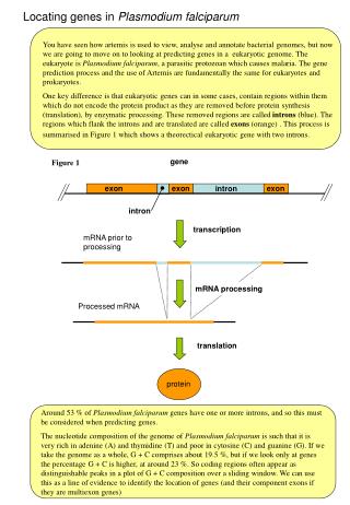
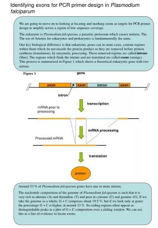
gene exon exon exon intron intron transcription mRNA prior to processing mRNA processing Processed mRNA translation protein Identifying exons for PCR primer design in Plasmodiumfalciparum We are going to move on to looking at locating and marking exons as targets for PCR primer design to amplify across a region of low sequence coverage. The eukaryote is Plasmodiumfalciparum, a parasitic protozoan which causes malaria. The The use of Artemis for eukaryotes and prokaryotes is fundamnentally the same. One key biological difference is that eukaryotic genes can in some cases, contain regions within them which do not encode the protein product as they are removed before protein synthesis (translation), by enzymatic processing. These removed regions are called introns (blue). The regions which flank the introns and are translated are called exons (orange). This process is summarised in Figure 1 which shows a theoretical eukaryotic gene with two introns. Figure 1 Around 53 % of Plasmodiumfalciparum genes have one or more introns. The nucleotide composition of the genome of Plasmodiumfalciparum is such that it is very rich in adenine (A) and thymidine (T) and poor in cytosine (C) and guanine (G). If we take the genome as a whole, G + C comprises about 19.5 %, but if we look only at genes the percentage G + C is higher, at around 23 %. So coding regions often appear as distinguishable peaks in a plot of G + C composition over a sliding window. We can use this as a line of evidence to locate exons.
The exact locations of exon/intron boundaries (also referred to as splice sites) is helped by the fact that they have particular sequence patterns (see Figure 2, see also Appendix IV). These patterns have a biological function as recognition signals to the cellular machinery that removes introns during RNA processing. We can identify these sequences by eye, or train computers to identify them. Note: The first two bases of the intron are always GT and the last two bases always AG. The others may vary. . .AAGGTAAAGA . . . . .TTTAGNNN. . . .TTCCATTTCT . . . . .AAATCNNN. . exon intron exon Location of exon/intron boundaries in P. falciparum Figure 2 Sequence patterns at exon/intron boundaries in Plasmodium. falciparum. 5’ 3’ Exercise The aim is to examine a region of chromosome 6 of P. falciparum, find 2 missing genes missing by examining GC and Correlation Score graphs. Your genes will then be refined by comparing them to genes in the database. The second part of the exercise is to design PCR primers to the two genes that you have identified so that you can PCR the region between them where the sequence quality is poor. Note: It is useful to have an internet browser open in the background for viewing search results Firstly open the file MAL6.region in artemis. Use the slider on right hand side( arrowed 1) to get a view of the whole region as below. From the Graph drop down menu select ‘GC Content %’.Use the slider on the GC graph (arrowed 2) to a adjust the GC content window size. Do the genes that are marked have corresponding peaks in the CG trace? 2 1
Display the ‘CorrelationScores’ graph by selecting it from the the same ‘Graph’ drop down menu. What do you notice about the coloured traces in regions where genes are located? We are now going to look for 2 missing genes in this region bounded by the green bar (coordinates 4400 - 12000) on the basis of GC content, correlation scores and FASTA search results. One gene has a single intron and the other does not have an intron. Look for peaks in the GC trace which correspond with separation of the Correlation Score traces. Are there also corresponding gaps in the stop codons in any of the six frames? Once you have identified such a region mark up a CDS in the gap in the stop codons. You do this by rapidly double clicking the central (scrolling) mouse button when the cursor arrow is pointing at the gap between stop codons. Then select ‘Create New Feature From Base Range’ from the create drop down menu. Then select OK. A light-blue CDS will then be marked up in that frame and also listed in the feature list (lower panel). Go through and mark up CDS’s in places where you think exons comprising the two genes may be present. We can now ready to run a search on the amino acid sequence of our CDS to compare it with proteins in the databases.
Before moving on to searching we’ ll look at an example of how genes with introns are represented in Artemis. Look at PFF0550w. Note that the exons are linked by a kinked line and may be present in the same frame, as in the case for PFF0520w, or be located in different frames as in PFF0550w. PFF0550w is shown in the screenshot below. The sequence of the exon/intron boundaries is visible in the lower panel. The ‘GT’ at the 5’ end of the intron and the ‘AG’ at the 3’ end are marked and arrowed for clarity. If you’re curious, quickly check how the sequence at the boundaries compare with the sequences described in Appendix IV. intron start intron end Now we are ready to run searches on predicted CDS’s. This will allow us to compare predictions against genes already in the database and give us information to decide if the predicted CDS is really a gene. It will also give us information which will help in the location of exon/intron boundaries. To search your predicted CDS features against the database: Select it by clicking in it, this should result in a black line outlining the CDS. Select the ‘Run’ dropdown menu, and from it ‘Run fasta on selected features against’ and ‘% uniprot’. These searches may take a few minutes so be patient. You can run the searches simultaneously by selecting all your predicted features and selecting the above option. When the search is complete a box appears. Access the results by pressing ‘r’or by selecting ‘View’ then ‘Search results’ then ‘fastaresults’ from the drop down menu (for both the CDS feature must be selected). These results can be sent to a internet browser by choosing ‘Send to browser’ which gives you a convenient way to click between the hit and the alignment as they are bookmarked. Your search give you a list of similar proteins in the database as well as alignments against your query protein (ask a demonstrator if you want more details).
Now we are in a position to define the exons precisely. Compare information from the alignment with the region that you have marked up (it is convenient to have the results window open in front of Artemis). Alignments can tell you whether the CDS region you have defined is internal to the gene, extends beyond the start or end (both), or whether it is likely to contain an intron. In the example below the CDS matches a protein in the database from position 53, ‘VAVIA .. to the end of the gene, but the start of the gene is missing. We have found an exon of the gene. Move the CDS from position 1 (red arrow) back to position 2 (red arrow). Note that an ‘AG’ sequence (red arrow 3 and boxed white) is present just before the start of the exon (starts with) ‘VAVIA’ giving confidence that this is a real intron – exon boundary. If you have any questions on this ask a demonstator. 3 2 1 Repeat this process of integrating GC data, correlation scores and FASTA searches to define the remaining exon of this gene. Remember that it could be in the same or a different frame, and that the first bases of the intron should be ‘GT’. To show the start codons (vertical magenta bars) right click in the middle panel and click the start codons box. If your gene prediction contains an intron it is necessary to merge them to show that they are linked. Do this by first clicking to select adjacent exons. Then select the ‘Edit’ drop down menu, then click OK and OK again when prompted ‘deleteoldfeatures’. The merging process may cause the exon to shift frame as the exact exon/intron boundary may be within a codon. Go back and check that the intron starts with a ‘GT’ and ends with ‘AG. If necessary you adjust the boundaries by clicking and dragging the end of the exons in the lower frame panel. To check your predictions reveal the missing genes by selecting ‘File’ then ‘Readanentry’ and choose the file ‘excercise3.tab’
The second part of the exercise is to design PCR primers to the two genes that you have just defined in order to amplify the region between them. For the sake of this exercise we’ll assume that the region between them has low sequence coverage. Designing PCR primers in exons rather than intergenic regions (introns and regions between genes) is a recommendable approach to obtain a PCR primer that is specific. As intergenic regions often have regions of low complexity, i.e. where there are long tracts of A and T. Such regions of low complexity make PCR primers design difficult. Briefly examine some introns and integenic regions to satsify yourself that this statement is reasonable. Select regions that you think are appropriate for PCR primers. Mark them up as genes by selecting ‘Create new feature from base range’ then in the upper left corned select ‘gene’ in the drop down menu. Remember that one primer must be designed on the coding strand and the other on the complementary strand. Ask a demonstrator if you have any questions. Then estimate the approximate size of the PCR product.