Gauges, Surface and NWP data
300 likes | 417 Views
Gauges, Surface and NWP data. Working Group summary slides June 29, 2005. How to organize?. By special emphases/interests Basic areas from Steve V. By individual data type By description of existing ‘systems’ Some combination. Aspects of Gauge data? .

Gauges, Surface and NWP data
E N D
Presentation Transcript
Gauges, Surface and NWP data Working Group summary slides June 29, 2005
How to organize? • By special emphases/interests • Basic areas from Steve V. • By individual data type • By description of existing ‘systems’ • Some combination
Aspects of Gauge data? • Data types, equipment, communications • Relative accuracies, reliabilities • Effective ranges of coverage, densities, issues of scale • Mesonets • Quality control strategies, in real-time and in retrospect • Historical versus real-time (operational) datasets • Archive availabilities
Aspects of Surface data? • Classic meteorologic synoptic variables at observing stations • Temperature, moisture, winds, pressure, etc. • derived, interpreted • vertical soundings, profiles (observed, remotely-sensed, modeled,?); surface transects; time-height plots; etc. • climatologic fields • categorical (targeted) climatologies • hydrologic observations • stage & flow observations • stage mesonets with level loggers • Availability/consistency of integrated Surface Analyses • Usage for regime typing and categorization
Aspects of NWP data? • Particular models, fields, characteristics • Deterministic, ensembled traces • Resolutions in time-space • Direct model usage vs. diagnostic usage • Utility for observation/forecast/updating • Downscaling approaches • Simplified (process) models • Data assimilation systems • Rapid refresh models • Coupled models (e.g., atmospheric-hydrologic) • Application/Utility-specific requirements for model output
Special Emphases • Hydromet Inputs over mountains for River Forecasting (PP, TA, HZ) • The utility of hydroclimatology in hydrometeorology • Fundamental Issues of ‘representative’ scale and resolution • NWP & surface analyses for regime typing • Gauge QC methods; manual & auto • Bias adjustment w/ gauges & r.s./NWP/surface data (& vice versa) • Oklahoma Mesonets • Modernizing the Cooperative Network • Archival & availability; real-time vs reanalysis • NCDC and real-time/meta- data archiving
Areas suggested by Steve • Analysis methods for Gauge data • current methods • MM, Oklahoma Mesonet, Neron • regional approaches • e.g., as mentioned, in the West, NWS River Forecast Centers (RFC’s) have used systems such as MM, with climatologic scaling based on PRISM (Daly et al, at Oregon State University) • I know there a number of other regional/local/commercial systems (e.g., P3 in Tulsa?) • Gauge QC methods • Use of sfc, r.s., NWP data to identify storm type, characteristics, etc. • e.g., research to include regime characterization into analysis algorithms and strategies; one example is an ongoing effort at synoptic regime (targeted) versions of the PRISM climatologies by Daly and the Oregon Climate Service with the NWS Western Region. • How to quantify Gauge uncertainty • Real-time calibration with Gauge data • RFC datasets as real-time components for Q2
Ed’s comments on ‘representativeness’ • Does Gauge QC matter? • Importance of QC for model verification • ETA 12 hour forecasts • WRF verification • Manual datasets and zeros • Business case for QC as a priority
Analysis Methods for QC • Current Methods • Regional example • Mountain Mapper
Hydromet Input Development in Complex Terrain • Common treatment of Observed & Future, R.T & historical: • Mean Areal Precipitation distribution (MAP) • Mean Areal Temperature distribution (MAT) • Mean Areal Snow/Freezing Level (‘MAZ’) • Complications • Extreme Non-stationarity/heterogeneity of fields • Phase changes with elevation • Limited effectiveness of remote sensors • Advantages • High Consistency across time-space scales • Good Atmospheric Model performance • Background Commonality • Climatology (PRISM)
Inversions in the West: data priority pyramid • Remote sensors • Surface datasets • Atmospheric models • Climatologies • Gauges
Mountain Mapper (MM) System: Quantitative Precipitation Development • QC-DAILY: QP Estimation (QPE) w/ Observed Data • QC of gauge reports • neighbor estimations via ‘normalized’ data • Gridded estimation of MAPs • RFS ingestion in real-time • problems with discontiguous areas with MAPX • Historical analysis/calibration • Freezing Level Estimation • Explicit Rain vs Snow delineation in RFS • Assist QC of observed data (e.g..., tipping bucket) • SPECIFY: QP Forecast (QPF) specification • VERIFY: QPF/QPE verification • ITERATE: MAP Analysis/Update/Iteration
Complimentary Data Types in Daily_QC • Surface Temperature • QC of gauge reports • Normalize/scale reports with climatology • neighbor estimations with differences (vs ratios with PP) • Gridded estimation of Temperature • PRISM max/min Temperature climatology grids • Display of basin aggregated MATs • Implicit Freezing Level Estimation • Currently: Lapsed for Rain/Snow delineation in RFS • Assist QC of observed data (e.g..., tipping bucket) • Snowmelt energy exchange • Freezing (Snow) Level heights • ‘observations’ from RUC analysis field • PAC-Jet Profilers • Simple (flat) Interpolation (no scaling)
n W i i=1 P x n W i i=1 1 W = 2 i d POINTS (stations) Estimating Precipitation Catch at station with missing report (P ) from surrounding observations (P ) B A C x i E D ( ) N P F x i N i = d= distance of separation W= station weight N= station seasonal mean P= station precip catch where
B A C E D F n P W i W i i=1 i P x n W i i=1 GRIDS LUMP POINTS PATTERN INTEGRATE Estimate grid boxes as “stations” ( ) 1 N x = 2 N i d = d= distance of separation
B A UPPER C E D LOWER F n P W i W i i=1 i P x n W i i=1 GRIDS LUMPS POINTS PATTERN INTEGRATE For each MAP area different for each season/month ( ) 1 N x = 2 N i d = d= distance of separation
MAP into SNOW MODEL SOIL MODEL BASIN RUNOFF MODEL (UNIT HYDROGRAPH) POINTS HRAP GRID * * Climatology: Seasonal or Monthly Isohyets QPF ----- * LUMP (MAP) ------------------
POINTS HRAP GRID 5500 ft 5500 ft * * QPF ----- Climatology: Seasonal or Monthly Isohyets Rain/snow 20 % SNOW 20% MAP into SNOW MODEL LUMP (MAP) ----------------- 80% RAIN 80% MAP into SOIL MODEL BASIN RUNOFF MODEL (UNIT HYDROGRAPH) Results in SMALLER Hydrograph
5500 ft 20 % SNOW Rain/snow elevation approximately 1000 feet below 0 C level (here, assume 1500 feet) o 80% RAIN Rain/snow E = E + (( T - PXTEMP) (100/L )) * rs v v p E = rain/snow elevation E = input variable elevation: freezing level or MAT T = input variable temperature: 0 C or MAT PXTEMP = threshold temperature [1 to 2 C] L = lapse rate during precipitation ( C/100m) [wet adiabatic or approx .55 C/100m or 3 F/1000 ft] rs v o v o o p o o
n W N i i i=1 n W i i=1 W i POINTS (stations) Estimating Temperature at a station with a missing report (T ) from surrounding observations (T ) B A x C i E D ( ( ) ) T F + - N i * x T = x d= distance of separation W= station weight N= station monthly mean T= station Temperature Fe= elevation factor E= elevation where 1 = d + Fe * E ix x ix
Works well but Obstacles include: • Timeliness: • Computational Speed • Communications • Human interactions • Software Tools • Non-orographic events • Once you’ve got the hammer, everything looks like a nail
Baseline is Improving:ongoing enhancements • Targeted (non-static) backgrounds for normalization • E.g., Ongoing development of Smart-PRISM (regime-sensitive) climatologies (Daly, Taylor group at Oregon State) • Atmospheric/process model data inclusion • Higher Spatial/Temporal resolutions • Iterative updating • Increased automation
Gauge QC methods/tests • Gross range checks • Nearest neighbor estimation (x-validation) • Gage history • Visual inspection of accumulation trace • Measuring Hardware: tipping vs. weighing; shielded? • Station network characteristics (SNOTEL, ASOS, etc.) • Station Measuring Hardware: tipping vs. weighing • Location wrt Freezing (Snow) Level • Disqualify tipping buckets
More Gauge QC methods/tests • Compare w/ SWE increment at co-located pillow (substitute) • Compare with remotely sensed data • NEXRAD overlay • IR Satellite views • Lightning strikes • Consider synoptic regime and surface data (e.g., post frontal convection?) • Adjust deviation allowed from neighbor estimation • Reasonableness of Gridded (hrap)/Basin (MAP) renditions of data • Consult longer duration results (monthly/seasonal performance w/ monthly-qc) • Consistency with temperature, freezing level, soil moisture
Identification of Synoptic Regime • Automated production from NWP/R.S./surface data • Adequate skill? • At what resolutions • Hourly • 5 km • Recommendations for prototyping
Quantifying Gage Uncertainty • Research topic • Indications from operational archive of meta-data • Results from multiple tests • Utility of Hydrologic application
Real-time role for RFC’s/mesonets in Q2 • Gauge QC stream as output • 6/24 hourly • 1 hourly progress • Availabilities • Real-time • Historical • Meta-data on QC • Validation, Bias adjustment • Regional Variations/Optimizations
Platform & Tools for ‘Community’ Model Development? • Accessible • Extensible • Consistent