
Fisher’s Exact Test
E N D
Presentation Transcript
Fisher’s Exact Test • Fisher’s Exact Test is a test for independence in a 2 X 2 table. It is most useful when the total sample size and the expected values are small. The test holds the marginal totals fixed and computes the hypergeometric probability that n11 is at least as large as the observed value • Useful when E(cell counts) < 5. EPI809/Spring 2008
Hypergeometric distribution • Example: 2x2 table with cell counts a, b, c, d. Assuming marginal totals are fixed: M1 = a+b, M2 = c+d, N1 = a+c, N2 = b+d. for convenience assume N1<N2, M1<M2. possible value of a are: 0, 1, …min(M1,N1). • Probability distribution of cell count a follows a hypergeometric distribution: N = a + b + c + d = N1 + N2 = M1 + M2 • Pr (x=a) = N1!N2!M1!M2! / [N!a!b!c!d!] • Mean (x) = M1N1/ N • Var (x) = M1M2N1N2 / [N2(N-1)] • Fisher exact test is based on this hypergeometric distr. EPI809/Spring 2008
Fisher’s Exact Test Example HIV Infection • Is HIV Infection related to Hx of STDs in Sub Saharan African Countries? Test at 5% level. Hx of STDs EPI809/Spring 2008
Hypergeometric prob. • Probability of observing this specific table given fixed marginal totals is Pr (3,7, 5, 10) = 10!15!8!17!/[25!3!7!5!10!] = 0.3332 • Note the above is not the p-value. Why? • Not the accumulative probability, or not the tail probability. • Tail prob = sum of all values (a = 3, 2, 1, 0). EPI809/Spring 2008
Hypergeometric prob Pr (2, 8, 6, 9) = 10!15!8!17!/[25!2!8!6!9!] = 0.2082 Pr (1, 9, 7, 8) = 10!15!8!17!/[25!1!9!7!8!] = 0.0595 Pr (0,10, 8, 7) = 10!15!8!17!/[25!0!10!8!7!] = 0.0059 Tail prob = .3332+.2082+.0595+.0059 = .6068 EPI809/Spring 2008
Fisher’s Exact Test SAS Codes Data dis; input STDs $ HIV $ count; cards; no no 10 No Yes 5 yes no 7 yes yes 3 ; run; proc freq data=dis order=data; weight Count; tables STDs*HIV/chisq fisher; run; EPI809/Spring 2008
Pearson Chi-squares test Yates correction • Pearson Chi-squares test χ2 = ∑i (Oi-Ei)2/Ei follows a chi-squares distribution with df = (r-1)(c-1) if Ei ≥ 5. • Yates correction for more accurate p-value χ2 = ∑i (|Oi-Ei| - 0.5)2/Ei when Oi and Ei are close to each other. EPI809/Spring 2008
Fisher’s Exact Test SAS Output Statistics for Table of STDs by HIV Statistic DF Value Prob ƒƒƒƒƒƒƒƒƒƒƒƒƒƒƒƒƒƒƒƒƒƒƒƒƒƒƒƒƒƒƒƒƒƒƒƒƒƒƒƒƒƒƒƒƒƒƒƒƒƒƒƒƒƒ Chi-Square 1 0.0306 0.8611 Likelihood Ratio Chi-Square 1 0.0308 0.8608 Continuity Adj. Chi-Square 1 0.0000 1.0000 Mantel-Haenszel Chi-Square 1 0.0294 0.8638 Phi Coefficient -0.0350 Contingency Coefficient 0.0350 Cramer's V -0.0350 WARNING: 50% of the cells have expected counts less than 5. Chi-Square may not be a valid test. Fisher's Exact Test ƒƒƒƒƒƒƒƒƒƒƒƒƒƒƒƒƒƒƒƒƒƒƒƒƒƒƒƒƒƒƒƒƒƒ Cell (1,1) Frequency (F) 10 Left-sided Pr <= F 0.6069 Right-sided Pr >= F 0.7263 Table Probability (P) 0.3332 Two-sided Pr <= P 1.0000 EPI809/Spring 2008
Fisher’s Exact Test • The output consists of three p-values: • Left: Use this when the alternative to independence is that there is negative association between the variables. That is, the observations tend to lie in lower left and upper right. • Right: Use this when the alternative to independence is that there is positive association between the variables. That is, the observations tend to lie in upper left and lower right. • 2-Tail: Use this when there is no prior alternative. EPI809/Spring 2008
Useful Measures of Association - Nominal Data • Cohen’s Kappa ( ) • Also referred to as Cohen’s General Index of Agreement. It was originally developed to assess the degree of agreement between two judges or raters assessing n items on the basis of a nominal classification for 2 categories. Subsequent work by Fleiss and Light presented extensions of this statistic to more than 2 categories. EPI809/Spring 2008
Inspector A Good Bad .40 (pB) Good Inspector ‘B’ .60 (qB) Bad .46 .54 1.00 (pA) (qA) Useful Measures of Association - Nominal Data • Cohen’s Kappa ( ) EPI809/Spring 2008
Useful Measures of Association - Nominal Data • Cohen’s Kappa ( ) • Cohen’s requires that we calculate two values: • po : the proportion of cases in which agreement occurs. In our example, this value equals 0.80. • Pe : the proportion of cases in which agreement would have been expected due purely to chance, based upon the marginal frequencies; where pe = pApB + qAqB = 0.508 for our data EPI809/Spring 2008
po - pe = = 0.593 1 - pe Useful Measures of Association - Nominal Data • Cohen’s Kappa ( ) • Then, Cohen’s measures the agreement between two variables and is defined by EPI809/Spring 2008
1 k = pe + pe2 - pi.p.i (pi.+p.i) (1 - pe) n i = 1 Useful Measures of Association - Nominal Data • Cohen’s Kappa ( ) • To test the Null Hypothesis that the true kappa = 0, we use the Standard Error: • then z = /~N(0,1) where pi. & p.i refer to row and column proportions (in textbook, ai= pi. & bi=p.i) EPI809/Spring 2008
Useful Measures of Association - Nominal Data- SAS CODES Data kap; input B $ A $ prob; n=100; count=prob*n; cards; Good Good .33 Good Bad .07 Bad Good .13 Bad Bad .47 ; run; procfreq data=kap order=data; weight Count; tables B*A/chisq; test kappa; run; EPI809/Spring 2008
Useful Measures of Association - Nominal Data- SAS OUTPUT The FREQ Procedure Statistics for Table of B by A Simple Kappa Coefficient ƒƒƒƒƒƒƒƒƒƒƒƒƒƒƒƒƒƒƒƒƒƒƒƒƒƒƒƒƒƒƒƒ Kappa 0.5935 ASE 0.0806 95% Lower Conf Limit 0.4356 95% Upper Conf Limit 0.7514 Test of H0: Kappa = 0 ASE under H0 0.0993 Z 5.9796 One-sided Pr > Z <.0001 Two-sided Pr > |Z| <.0001 Sample Size = 100 EPI809/Spring 2008
McNemar’s Test for Correlated (Dependent) Proportions EPI809/Spring 2008
McNemar’s Test for Correlated (Dependent) Proportions Basis / Rationale for the Test • The approximate test previously presented for assessing a difference in proportions is based upon the assumption that the two samples are independent. • Suppose, however, that we are faced with a situation where this is not true. Suppose we randomly-select 100 people, and find that 20% of them have flu. Then, imagine that we apply some type of treatment to all sampled peoples; and on a post-test, we find that 20% have flu. EPI809/Spring 2008
McNemar’s Test for Correlated (Dependent) Proportions • We might be tempted to suppose that no hypothesis test is required under these conditions, in that the ‘Before’ and ‘After’ p values are identical, and would surely result in a test statistic value of 0.00. • The problem with this thinking, however, is that the two sample p values are dependent, in that each person was assessed twice. It is possible that the 20 people that had flu originally still had flu. It is also possible that the 20 people that had flu on the second test were a completely different set of 20 people! EPI809/Spring 2008
McNemar’s Test for Correlated (Dependent) Proportions • It is for precisely this type of situation that McNemar’s Test for Correlated (Dependent) Proportions is applicable. • McNemar’s Test employs two unique features for testing the two proportions: * a special fourfold contingency table; with a * special-purpose chi-square (2) test statistic (the approximate test). EPI809/Spring 2008
where (A+B) + (C+D) = (A+C) + (B+D) = n = number of units evaluated and where df = 1 A B (A + B) C D (C + D) (A + C) (B + D) n McNemar’s Test for Correlated (Dependent) Proportions Nomenclature for the Fourfold (2 x 2) Contingency Table EPI809/Spring 2008
McNemar’s Test for Correlated (Dependent) Proportions 1. Construct a 2x2 table where the paired observations are the sampling units. 2. Each observation must represent a single joint event possibility; that is, classifiable in only one cell of the contingency table. 3. In it’s Exact form, this test may be conducted as a One Sample Binomial for the B & C cells Underlying Assumptions of the Test EPI809/Spring 2008
McNemar’s Test for Correlated (Dependent) Proportions • 4. The expected frequency (fe) for the B and C cells on the contingency table must be equal to or greater than 5; where fe = (B + C) / 2 from the Fourfold table Underlying Assumptions of the Test EPI809/Spring 2008
McNemar’s Test for Correlated (Dependent) Proportions Sample Problem A randomly selected group of 120 students taking a standardized test for entrance into college exhibits a failure rate of 50%. A company which specializes in coaching students on this type of test has indicated that it can significantly reduce failure rates through a four-hour seminar. The students are exposed to this coaching session, and re-take the test a few weeks later. The school board is wondering if the results justify paying this firm to coach all of the students in the high school. Should they? Test at the 5% level. EPI809/Spring 2008
McNemar’s Test for Correlated (Dependent) Proportions Sample Problem The summary data for this study appear as follows: EPI809/Spring 2008
Before Pass Fail Pass 56 56 112 After Fail 4 4 8 60 60 120 McNemar’s Test for Correlated (Dependent) Proportions The data are then entered into the Fourfold Contingency table: EPI809/Spring 2008
McNemar’s Test for Correlated (Dependent) Proportions • Step I : State the Null & Research Hypotheses H0 : 1 = 2 H1 : 1 2 where 1 and 2relate to the proportion of observations reflecting changes in status (the B & C cells in the table) • Step II : = 0.05 EPI809/Spring 2008
{ ABS (B - C) - 1 }2 2 = B + C McNemar’s Test for Correlated (Dependent) Proportions • Step III : State the Associated Test Statistic EPI809/Spring 2008
McNemar’s Test for Correlated (Dependent) Proportions • Step IV : State the distribution of the Test Statistic When Ho is True 2 = 2 with 1 df when Ho is True d EPI809/Spring 2008
X² Distribution Chi-Square Curve w. df=1 0 X² 3.84 McNemar’s Test for Correlated (Dependent) Proportions Step V : Reject Ho if ABS ( 2 ) > 3.84 EPI809/Spring 2008
{ ABS (56 - 4) - 1 }2 2 = = 43.35 56 + 4 McNemar’s Test for Correlated (Dependent) Proportions • Step VI : Calculate the Value of the Test Statistic EPI809/Spring 2008
McNemar’s Test for Correlated (Dependent) Proportions-SAS Codes Data test; input Before $ After $ count; cards; pass pass 56 pass fail 56 fail pass 4 fail fail 4; run; procfreq data=test order=data; weight Count; tables Before*After/agree; run; EPI809/Spring 2008
McNemar’s Test for Correlated (Dependent) Proportions-SAS Output Statistics for Table of Before by After McNemar's Test ƒƒƒƒƒƒƒƒƒƒƒƒƒƒƒƒƒƒƒƒƒƒƒƒ Statistic (S) 45.0667 DF 1 Pr > S <.0001 Sample Size = 120 Without the correction EPI809/Spring 2008
Conclusion: What we have learned • Comparison of binomial proportion using Z and 2 Test. • Explain 2 Test for Independence of 2 variables • Explain The Fisher’s test for independence • McNemar’s tests for correlated data • Kappa Statistic • Use of SAS Proc FREQ EPI809/Spring 2008
Conclusion: Further readings Read textbook for • Power and sample size calculation • Tests for trends EPI809/Spring 2008