Download

1 / 62
630 likes | 792 Views
Constraint Satisfaction and Backtrack Search 22c:31 Algorithms. Overview. Constraint Satisfaction Problems (CSP) share some common features and have specialized methods

E N D
Overview • Constraint Satisfaction Problems (CSP) share some common features and have specialized methods • View a problem as a set of variables to which we have to assign values that satisfy a number of problem-specific constraints. • Constraint solvers, constraint logic programming… • Algorithms for CSP • Backtracking (systematic search) • Variable ordering heuristics • Backjumping and dependency-directed backtracking
Informal Definition of CSP • CSP = Constraint Satisfaction Problem • Given (V, D, C) (1) V: a finite set of variables (2) D: a domain of possible values (often finite) (3) C: a set of constraints that limit the values the variables can take on • A solution is an assignment of a value to each variable such that all the constraints are satisfied. • Tasks might be to decide if a solution exists, to find a solution, to find all solutions, or to find the “best solution” according to some metric f.
Example: Path of Length k • Given an undirected graph G = (V, E), does G have a simple path of length k? • Variables: x1, x2, …, xk • Domain of variables: V • Constraints: • (a) all values to xi are distinct; • (b) (xi xi+1) is in E.
Example: Clique of Size k • Given an undirected graph G = (V, E), does G have a vertex cover of size k? • Variables: X = { x1, x2, …, xk } • Domain of variables: V • Constraints: • (a) all values to xi are distinct; • (b) (xi xj) is in E for any i and j.
Example: Vertex Cover of Size k • Given an undirected graph G = (V, E), does G have a clique of size k? • Variables: X = { x1, x2, …, xk } • Domain of variables: V • Constraints: • (a) all values to xi are distinct; • (b) For each edge (a, b) of E, a or b is in X.
Example: Isomorphic Graphs • Given two undirected graph G = (V, E), and H = (U, D), where |V| = |U|, does there is a one-to-one mapping f : V -> U, such that f(E) = D? • Variables: X = { f(v) | v in V } • Domain of variables: V • Constraints: • (a) all values to f(v) are distinct; • (b) |E| = |D| and for each edge (a, b) of E, (f(a) f(b)) is in D.
Example: Permutations of a Set • Given a set S of n elements, print all the permutations of S. • Variables: X = { xi | 1 <= i <= n } • Domain of variables: S • Constraints: • all values to xi are distinct.
Example: Permutations of a Set • Given a set S of n elements, print all the permutations of S. • Variables: X = { xi | 1 <= i <= n } • Domain of variables: S • Constraints: • all values to xi are distinct. Perm(m, n, X) { if (m == 0) { print(X, n); return; } for (y = 1; y <= n; y++) { if not(y in X[m+1..n]) { X[k] = y; Perm(m – 1, n, X); } } } First call: Perm(n, n, X)
Example: Combinations of k elements from a Set • Given a set S of n elements, print all combinations of k elements of S. • Variables: X = { xi | 1 <= i <= k < n } • Domain of variables: S • Constraints: x1 < x2 < x3 < … < xk
Example: Combinations of k elements from a Set • Given a set S of n elements, print all combinations of k elements of S. • Variables: X = { xi | 1 <= i <= k < n } • Domain of variables: S • Constraints: x1 < x2 < x3 < … < xk Combin(k, m, n, X) { if (k == 0) { print(X, n); return; } for (y = k; y <= m; y++) { X[k] = y; Combin(k – 1, y – 1, n, X); } } First call: Combin(k, n, n, X)
SEND + MORE = MONEY Assign distinct digits to the letters S, E, N, D, M, O, R, Y such that S E N D + M O R E = M O N E Y holds.
SEND + MORE = MONEY Solution 9 5 6 7 + 1 0 8 5 = 1 0 6 5 2 Assign distinct digits to the letters S, E, N, D, M, O, R, Y such that S E N D + M O R E = M O N E Y holds.
Modeling Formalize the problem as a CSP: • Variables: v1,…,vn • Domains: Z, integers • Constraints: c1,…,cm n • problem: Find a =(v1,…,vn) nsuch that a ci , for all 1 i m
A Model for MONEY • variables: { S,E,N,D,M,O,R,Y} • constraints: c1={(S,E,N,D,M,O,R,Y) 8 | 0 S,…,Y 9 } c2={(S,E,N,D,M,O,R,Y) 8 | 1000*S + 100*E + 10*N + D + 1000*M + 100*O + 10*R + E = 10000*M + 1000*O + 100*N + 10*E + Y}
A Model for MONEY(continued) • more constraints c3= {(S,E,N,D,M,O,R,Y) 8 | S 0 } c4= {(S,E,N,D,M,O,R,Y) 8 | M 0 } c5= {(S,E,N,D,M,O,R,Y) 8 | S…Y all different}
Solution for MONEY c1={(S,E,N,D,M,O,R,Y) 8 | 0S,…,Y9 } c2={(S,E,N,D,M,O,R,Y) 8 | 1000*S + 100*E + 10*N + D + 1000*M + 100*O + 10*R + E = 10000*M + 1000*O + 100*N + 10*E + Y} c3= {(S,E,N,D,M,O,R,Y) 8 | S 0 } c4= {(S,E,N,D,M,O,R,Y) 8 | M 0 } c5= {(S,E,N,D,M,O,R,Y) 8 | S…Y all different} Solution: (9,5,6,7,1,0,8,2)8
E D A B C Example: Map Coloring • Color the following map using three colors (red, green, blue) such that no two adjacent regions have the same color.
E E D A B D A B C C Example: Map Coloring • Variables: A, B, C, D, E all of domain RGB • Domains: RGB = {red, green, blue} • Constraints: AB, AC,A E, A D, B C, C D, D E • One solution: A=red, B=green, C=blue, D=green, E=blue =>
N-queens Example (4 in our case) • Standard test case in CSP research • Variables are the rows: r1, r2, r3, r4 • Values are the columns: {1, 2, 3, 4} • So, the constraints include: • Cr1,r2 = {(1,3),(1,4),(2,4),(3,1),(4,1),(4,2)} • Cr1,r3 = {(1,2),(1,4),(2,1),(2,3),(3,2),(3,4), (4,1),(4,3)} • Etc. • What do these constraints mean?
Example: SATisfiability • Given a set of propositional variables and Boolean formulas, find an assignment of the variables to {false, true} that satisfies the formulas. • Example: • Boolean variables = { A, B, C, D} • Boolean formulas: A \/ B \/ ~C, ~A \/ D, B \/ C \/ D • (the first two equivalent to C -> A \/ B, A -> D) • Are satisfied by A = false B = true C = false D = false
Scheduling Temporal reasoning Building design Planning Optimization/satisfaction Vision Graph layout Network management Natural language processing Molecular biology / genomics VLSI design Real-world problems
Formal definition of a CSP A constraint satisfaction problem (CSP) consists of • a set of variables X = {x1, x2, … xn} • each with an associated domain of values {d1, d2, … dn}. • The domains are typically finite • a set of constraints {c1, c2 … cm} where • each constraint defines a predicate which is a relation over a particular subset of X. • E.g., Ci involves variables {Xi1, Xi2, … Xik} and defines the relation Ri Di1 x Di2 x … Dik
Formal definition of a CSP • Instantiations • An instantiation of a subset of variables S is an assignment of a domain value to each variable in in S • An instantiation is legal iff it does not violate any (relevant) constraints. • A solution is a legal instantiation of all of the variables in the network.
Typical Tasks for CSP • Solutions: • Does a solution exist? • Find one solution • Find all solutions • Given a partial instantiation, do any of the above • Transform the CSP into an equivalent CSP that is easier to solve.
Constraint Solving is Hard Constraint solving is not possible for general constraints. Example (Fermat’s Last Theorem): C: n > 2 C’: an + bn = cn Constraint programming separates constraints into • basic constraints: complete constraint solving • non-basic constraints: propagation (incomplete); search needed
CSP as a Search Problem States are defined by the values assigned so far • Initial state: the empty assignment { } • Successor function: assign a value to an unassigned variable that does not conflict with current assignment fail if no legal assignments • Goal test: the current assignment is complete • This is the same for all CSPs • Every solution appears at depth n with n variables use depth-first search with backtrack • Path is irrelevant, so can also use complete-state formulation • Local search methods are useful.
Systematic search: Backtracking(backtrack depth-first search) • Consider the variables in some order • Pick an unassigned variable and give it a provisional value such that it is consistent with all of the constraints • If no such assignment can be made, we’ve reached a dead end and need to backtrack to the previous variable • Continue this process until a solution is found or we backtrack to the initial variable and have exhausted all possible values. • DFS: When backtrack, a node is marked as “processed” • CSP: When backtrack, a node is unmarked as “ discovered”
Backtracking search • Variable assignments are commutative, i.e., [ A = red then B = green ] same as [ B = green then A = red ] • Only need to consider assignments to a single variable at each node b = d and there are dn leaves • Depth-first search for CSPs with single-variable assignments is called backtracking search • Backtracking search is the basic algorithm for CSPs • Can solve n-queens for n≈ 100
S N E N N N D N M N O N R N Y N S E N D+ M O R E= M O N E Y 0S,…,Y9 S 0 M 0 S…Y all different 1000*S + 100*E + 10*N + D + 1000*M + 100*O + 10*R + E = 10000*M + 1000*O + 100*N + 10*E + Y
Propagate S E N D+ M O R E= M O N E Y S {0..9} E {0..9} N {0..9} D {0..9} M {0..9} O {0..9} R {0..9} Y {0..9} 0S,…,Y9 S 0 M 0 S…Y all different 1000*S + 100*E + 10*N + D + 1000*M + 100*O + 10*R + E = 10000*M + 1000*O + 100*N + 10*E + Y
Propagate S E N D+ M O R E= M O N E Y S {1..9} E {0..9} N {0..9} D {0..9} M {1..9} O {0..9} R {0..9} Y {0..9} 0S,…,Y9 S 0 M 0 S…Y all different 1000*S + 100*E + 10*N + D + 1000*M + 100*O + 10*R + E = 10000*M + 1000*O + 100*N + 10*E + Y
Propagate S E N D+ M O R E= M O N E Y S {9} E {4..7} N {5..8} D {2..8} M {1} O {0} R {2..8} Y {2..8} 0S,…,Y9 S 0 M 0 S…Y all different 1000*S + 100*E + 10*N + D + 1000*M + 100*O + 10*R + E = 10000*M + 1000*O + 100*N + 10*E + Y
Branch S {9} E {4..7} N {5..8} D {2..8} M {1} O {0} R {2..8} Y {2..8} S E N D+ M O R E= M O N E Y 0S,…,Y9 S 0 M 0 S…Y all different 1000*S + 100*E + 10*N + D + 1000*M + 100*O + 10*R + E = 10000*M + 1000*O + 100*N + 10*E + Y E 4 E = 4 S {9} E {4} N {5} D {2..8} M {1} O {0} R {2..8} Y {2..8} S {9} E {5..7} N {6..8} D {2..8} M {1} O {0} R {2..8} Y {2..8}
Propagate S {9} E {4..7} N {5..8} D {2..8} M {1} O {0} R {2..8} Y {2..8} S E N D+ M O R E= M O N E Y 0S,…,Y9 S 0 M 0 S…Y all different 1000*S + 100*E + 10*N + D + 1000*M + 100*O + 10*R + E = 10000*M + 1000*O + 100*N + 10*E + Y E 4 E = 4 S {9} E {5..7} N {6..8} D {2..8} M {1} O {0} R {2..8} Y {2..8}
Branch S {9} E {4..7} N {5..8} D {2..8} M {1} O {0} R {2..8} Y {2..8} S E N D+ M O R E= M O N E Y E 4 E = 4 S {9} E {5..7} N {6..8} D {2..8} M {1} O {0} R {2..8} Y {2..8} E = 5 E 5 S {9} E {6..7} N {6..8} D {2..8} M {1} O {0} R {2..8} Y {2..8} S {9} E {5} N {6} D {2..8} M {1} O {0} R {2..8} Y {2..8}
Propagate S {9} E {4..7} N {5..8} D {2..8} M {1} O {0} R {2..8} Y {2..8} S E N D+ M O R E= M O N E Y E 4 E = 4 S {9} E {5..7} N {6..8} D {2..8} M {1} O {0} R {2..8} Y {2..8} E = 5 E 5 S {9} E {5} N {6} D {7} M {1} O {0} R {8} Y {2} S {9} E {6..7} N {7..8} D {2..8} M {1} O {0} R {2..8} Y {2..8}
Complete Search Tree S {9} E {4..7} N {5..8} D {2..8} M {1} O {0} R {2..8} Y {2..8} S E N D+ M O R E= M O N E Y E = 4 E 4 S {9} E {5..7} N {6..8} D {2..8} M {1} O {0} R {2..8} Y {2..8} E = 5 E 5 S {9} E {5} N {6} D {7} M {1} O {0} R {8} Y {2} S {9} E {6..7} N {7..8} D {2..8} M {1} O {0} R {2..8} Y {2..8} E 6 E = 6
Problems with backtracking • Thrashing: keep repeating the same failed variable assignments • Consistency checking can help • Intelligent backtracking schemes can also help • Inefficiency: can explore areas of the search space that aren’t likely to succeed • Variable ordering can help
Improving backtracking efficiency • General-purpose methods can give huge gains in speed: • Which variable should be assigned next? • In what order should its values be tried? • Can we detect inevitable failure early?
Most constrained variable • Most constrained variable: choose the variable with the fewest legal values • a.k.a. minimum remaining values (MRV) heuristic
Most constraining variable • Tie-breaker among most constrained variables • Most constraining variable: • choose the variable with the most constraints on remaining variables
Least constraining value • Given a variable, choose the least constraining value: • the one that rules out the fewest values in the remaining variables • Combining these heuristics makes 1000 queens feasible
Symmetry Breaking Often, the most efficient model admits many different solutions that are essentially the same (“symmetric” to each other). Symmetry breaking tries to improve the performance of search by eliminating such symmetries.
E E D A B D A B C C Example: Map Coloring • Variables: A, B, C, D, E all of domain RGB • Domains: RGB = {red, green, blue} • Constraints: AB, AC,A E, A D, B C, C D, D E • One solution: A=red, B=green, C=blue, D=green, E=blue =>