Download
1 / 47
470 likes | 602 Views
This article delves into the concept of the regression equation, focusing on how it enables personalized predictions rather than relying solely on average outcomes. It examines the best-fitting line, characterized as minimizing the average squared distance of Y scores from this line, and presents the generic formula Y = mx + b. The article highlights the significance of correlation coefficients and differentiates between sample predictions and population estimates. Finally, it emphasizes the importance of careful use of individualized predictions to avoid increasing error in statistical modeling.

E N D
The Regression Equation Using the regression equation to individualize prediction and move beyond saying that everyone is equal, that everyone should score right at the mean
The definition of the best fitting line plotted on t axes • A “best fitting line” minimizes the average squared vertical distance of Y scores in the sample (expressed as tY scores) from the line. • The best fitting line is a least squares, unbiased estimate of values of Y in the sample. • The generic formula for a line is Y=mx+b where m is the slope and b is the Y intercept. • Thus, any specific line, such as the best fitting line, can be defined by its slope and its intercept.
The intercept of the best fitting line plotted on t axes The origin is the point where both tX and tY=0.000 • So the origin represents the mean of both the X and Y variable • When plotted on t axes all best fitting lines go through the origin. • Thus, the tYintercept of the best fitting line = 0.000.
The slope of and formula for the best fitting line • When plotted on t axes the slope of the best fitting line = r, the correlation coefficient. • To define a line we need its slope and Y intercept • r = the slope and tY intercept=0.00 • The formula for the best fitting line is therefore tY=rtX + 0.00 or tY= rtX
Here’s how a visual representation of the best fitting line (slope = r, Y intercept = 0.000) and the dots representing tX and tY scores might be described. (Whether the correlation is positive of negative doesn’t matter.) • Perfect - scores fall exactly on a straight line. • Strong - most scores fall near the line. • Moderate - some are near the line, some not. • Weak - the scores are only mildly linear. • Independent - the scores are not linear at all.
1.5 Perfect 1.0 0.5 -1.5 -1.0 -0.5 0 0.5 1.0 1.5 0 -0.5 -1.0 -1.5 Strength of a relationship
1.5 1.0 Strong r about .800 0.5 -1.5 -1.0 -0.5 0 0.5 1.0 1.5 0 -0.5 -1.0 -1.5 Strength of a relationship
1.5 1.0 0.5 -1.5 -1.0 -0.5 0 0.5 1.0 1.5 0 -0.5 -1.0 -1.5 Strength of a relationship Moderate r about .500
1.5 1.0 0.5 -1.5 -1.0 -0.5 0 0.5 1.0 1.5 0 -0.5 -1.0 Independent -1.5 Strength of a relationshipr about 0.000
1.5 1.0 0.5 -1.5 -1.0 -0.5 0 0.5 1.0 1.5 0 -0.5 -1.0 -1.5 r=.800, the formula for the best fitting line = ???
1.5 1.0 0.5 -1.5 -1.0 -0.5 0 0.5 1.0 1.5 0 -0.5 -1.0 -1.5 r=-.800, the formula for the best fitting line = ???
1.5 1.0 0.5 -1.5 -1.0 -0.5 0 0.5 1.0 1.5 0 -0.5 -1.0 -1.5 r=0.000, the formula for the best fitting line is:
Notice what that formula for independent variables says • tY = rtX = 0.000 (tX) = 0.000 • When tY = 0.000, you are at the mean of Y • So, when variables are independent, the best fitting line says that the best estimate of Y scores in the sample is back to the mean of Y regardless of your score on X • Thus, when variables are independent we go back to saying everyone will score right at the mean
1.5 1.0 0.5 -1.5 -1.0 -0.5 0 0.5 1.0 1.5 0 -0.5 -1.0 -1.5 A note of caution: Watch out for the plot for which the best fitting line is a curve.
Moving from the best fitting line to the regression equation and the regression line.
The best fitting line (tY=rtX) was the line closest to the Y values in the sample. But what should we do if we want to go beyond our sample and use a version of our best fitting line to make individualized predictions for the rest of the population?
What do we need to do to be able to use the regression equation • tY' = rtX • Notice this is not quite the same as the formula for the best fitting line. The formula now reads tY' (read t-y-prime). Not tY. • tY' is the predicted score on the Y variable for every X score in the population within the range observed in our random sample. • Before we were describing the linear relationship of the X and Y variable in our sample. Now we are predicting estimated Z scores (t scores) for most or all of the population.
This is one of the key points in the course; a point when things change radically. Up to this point, we have just been describing scores, means and relationships. We have not yet gone beyond predicting that everyone in the population who was not in our sample will score at the mean of Y. But now we want to be able to make individualized predictions for the rest of the population, the people not in our sample and for whom we don’t have Y scores
That’s dangerous. Our first rule as scientists in “Do not increase error.” Individualizing prediction can easily do that. Let me give you an example.
Assume, you are the personnel officer for a mid size company. • You need to hire a typist. • There are 2 applicants for the job. • You give the applicants a typing test. • Which would you hire: someone who types 6 words a minute with 12 mistakes or someone who types 100 words a minute with 1 mistake.
Who would you hire? • Of course, you would predict that the second person will be a better typist and hire that person. • Notice that we never gave the person with 6 words/minute a chance to be a typist in our firm. • We prejudged her on the basis of the typing test. • That is probably valid in this case – a typing test probably predicts fairly well how good a typist someone will be.
But say the situation is a little more complicated! • You have several applicants for a leadership position in your firm. • But it is not 2002, it is 1957, when we knew that only white males were capable of leadership in corporate America. • That is, we all “know” that leadership ability is correlated with both gender and skin color, white and male are associated with high leadership ability and darker skin color and female gender with lower leadership ability. • We now know this is absurd, but lots of people were never given a chance to try their hand at leadership, because of pre-judgement that you can now see as obvious prejudice.
We would have been much better off saying that everyone is equal, everyone should be predicted to score at the mean. • Pre-judgements on the basis of supposed relationships between variables that have no real scientific support are a form of prejudice. • They cost potential leaders jobs in which they could have shown their ability. That is unfair. • Moreover, by excluding such individuals, you narrow the talent pool of potential leaders. The more restricted the group of potential leaders, the less talented the average leader will be. • This is why aristocracies don’t work in the long run. The talent pool is too small.
So, to avoid prejudice you must start with the notion that everyone will score at the mean.In correlational language, to make that prediction you have to hypothesize that rho = 0.000.Only if you can disprove the notion that rho = 0.000 and no other time, should you make any other prediction
We call the hypothesis that rh0=0.000 the null hypothesis The symbol for the null hypothesis is H0. We will see the null hypothesis many times during the rest of this course. It is the hypothesis that you will learn to test statistically.
Confidence intervals around rhoT – relation to Chapter 6 • In Chapter 6 we learned to create confidence intervals around muT that allowed us to test a theory. • To test our theory about mu we took a random sample, computed the sample mean and standard deviation, and determined whether the sample mean fell into that interval. • If the sample mean fell into the confidence interval, there was some support for our theory, and we held onto it. • The interesting case was when muT fell outside the confidence interval. • In that case, the data from our sample falsified our theory, so we had to discard the theory and the estimate of mu specified by the theory
If we discard a theory based prediction, what do we use in its place? • Generally, our best estimate of a population parameter is the sample statistic that estimates it. • Our best estimate of mu has been and is the sample mean, X-bar. • Since X-bar fell outside the confidence interval, we discarded our theory. • Then we were back to using X-bar, the sample mean that fell outside the confidence interval and falsified our theory, as our best (least squares, unbiased, consistent estimate) of mu.
To test any theory about any population parameter, we go through similar steps: • We theorize about the value of the population parameter. • We obtain some measure of the variability of sample based estimates of the population parameter. • We create a test of the theory about the population parameter by creating a confidence interval, almost always a CI.95. • We then obtain and measure the parameter in a random sample.
The sample statistic will fall inside or outside of the CI.95 • If the sample statistic falls inside the confidence interval, our theory has received some support and we hold on to it. • But the more interesting case is when the sample statistic falls outside the confidence interval. • Then we must discard the theory and the theory based estimate of the population parameter. • In that case, our best estimate of the population parameter is the sample statistic • Remember, the sample statistic is a least squares, unbiased, consistent estimate of its population parameter.
We are going to do the same thing with a theory about rho • rho is the correlation coefficient for the population. • If we have a theory about rho, we can create a 95% confidence interval into which we expect r will fall. • An r computed from a random sample will then fall inside or outside the confidence interval.
When r falls inside or outside of the CI.95 around rhoT • If r falls inside the confidence interval, our theory about rho has received some support and we hold on to it. • But the more interesting case is when r falls outside the confidence interval. • Then we must discard the theory and the theory based estimate of the population parameter. • In that case, our best estimate of rho is the r we found in our random sample • Thus, when r falls outside the CI.95 we can go back to using it as a least squares unbiased estimate of rho.
Then what? • Then we can use the r from our sample, the r that falsified the theory that rho=0.000, in the regression equation: • tY'=rtX
To repeat • If rho = 0.000, we should go back to saying everyone is equal, everyone will score at the mean of Y. • To be fair and avoid doing damage, we must test the hypothesis that rho=0.000 before doing anything else. • To test the theory that rho=0.00, we create a CI.95 for rho=0.000. • If, and only if, we disprove the notion that rho=0.000 by having r fall outside the CI.95 can we use r in the regression equation, tY'=rtX.
I could teach you how to calculate the confidence interval for rho=0.000 • But other people have already calculated the intervals for many different df. • Those calculations are summarized in the r table
How the r table is laid out: the important columns • Column 1 of the r table shows degrees of freedom for correlation and regression (dfREG) • dfREG=nP-2 • Column 2 shows the CI.95 for varying degrees of freedom • Column 3 shows the absolute value of the r that falls just outside the CI.95. Any r this far or further from 0.000 falsifies the hypothesis that rho=0.000 and can be used in the regression equation to make predictions of Y scores for people who were not in the original sample but who were part of the population from which the sample is drawn.
If r falls in within the 95% CI around 0.000, then the result is not significant. df nonsignificant .05 .01 1 2 3 4 5 6 7 8 9 10 11 12 . . . 100 200 300 500 1000 2000 10000 -.996 to .996 -.949 to .949 -.877 to .877 -.810 to .810 -.753 to .753 -.706 to .706 -.665 to .665 -.631 to .631 -.601 to .601 -.575 to .575 -.552 to .552 -.531 to .531 . . . -.194 to .194 -.137 to .137 -.112 to .112 -.087 to .087 -.061 to .061 -.043 to .043 -.019 to .019 .997 .950 .878 .811 .754 .707 .666 .632 .602 .576 .553 .532 . . . .195 .138 .113 .088 .062 .044 .020 .9999 .990 .959 .917 .874 .834 .798 .765 .735 .708 .684 .661 . . . .254 .181 .148 .115 .081 .058 .026 Does the absolute value of r equal or exceed the value in this column? Find your degrees of freedom (Np-2) in this column You cannot reject the null hypothesis. You can use it in the regression equation to estimate Y scores. r is significant with alpha = .05. You must assume that rho = 0.00. If r is significant you can consider it an unbiased, least squares estimate of rho. alpha = .05.
Pizza and horror films horror films 7 9 8 6 9 6 5 2 1 6 (scale 0-9) anchovies 7 7 3 3 0 8 4 1 1 1 H1: People who enjoy food with strong flavors also enjoy other strong sensations. H0: There is no relationship between enjoying food with strong flavors and enjoying other strong sensations. Can we reject the null hypothesis?
8 6 4 2 0 0 2 4 6 8 Can we reject the null hypothesis? Pizza Horror films
Can we reject the null hypothesis? We do the math and we find that: r = .352 df = 8
df nonsignificant .05 .01 r table 1 2 3 4 5 6 7 8 9 10 11 12 . . . 100 200 300 500 1000 2000 10000 .997 .950 .878 .811 .754 .707 .666 .632 .602 .576 .553 .532 . . . .195 .138 .113 .088 .062 .044 .020 -.996 to .996 -.949 to .949 -.877 to .877 -.810 to .810 -.753 to .753 -.706 to .706 -.665 to .665 -.631 to .631 -.601 to .601 -.575 to .575 -.552 to .552 -.531 to .531 . . . -.194 to .194 -.137 to .137 -.112 to .112 -.087 to .087 -.061 to .061 -.043 to .043 -.019 to .019 .9999 .990 .959 .917 .874 .834 .798 .765 .735 .708 .684 .661 . . . .254 .181 .148 .115 .081 .058 .026
This finding falls within the CI.95 around 0.000 • We call such findings “nonsignificant” • Nonsignificant is abbreviated n.s. • We would report these finding as follows • r (8)=0.352, n.s. • Given that it fell inside the CI.95, we must assume that rho actually equals zero and that our sample r is not 0.000 solely because of sampling fluctuation. • We go back to predicting that everyone will score at the mean of Y.
That seems like a good idea: • I would guess that like most variables, desire for anchovy pizza and horror movies are not really correlated. • This sample probably has an r of .352 solely because of the way samples of this size fluctuate around a rho of zero
How to report a signficant r • For example, let’s say that you had a sample (nP=30) and r = -.400 • Looking under nP-2=28 dfREG, we find the interval consistent with the null is between -.360 and +.360 • So we are outside the CI.95 for rho=0.000 • We would write that result as r(28)=-.400, p<.05 • That tells you the dfREG, the value of r, and that you can expect an r that far from 0.000 five or fewer times in 100 when rho = 0.000
Then there is Column 4 • Column 4 shows the values that lie outside a CI.99 • (The CI.99 itself isn’t shown like the CI.95 in Column 2 because it isn’t important enough.) • However, Column 4 gives you bragging rights. • If your r is as far or further from 0.000 as the number in Column 4, you can say there is 1 or fewer chance in 100 of an r being this far from zero (p<.01). • For example, let’s say that you had a sample (nP=30) and r = -.525. • The critical value at .01 is .463. You are further from 0.00 than that.So you can brag. • You write that result as r(28)=-.525, p<.01.
To summarize • If r falls inside the CI.95 around 0.000, it is nonsignificant (n.s.) and you can’t use the regression equation (e.g., r(28)=.300, n.s. • If r falls outside the CI.95, but not as far from 0.000 as the number in Column 4, you have a significant finding and can use the regression equation (e.g., r(28)=-.400,p<.05 • If r is as far or further from zero as the number in Column 4, you can use the regression equation and brag while doing it (e.g., r(28)=-.525, p<.01