Understanding Distributions: Box Plots, Histograms, and Key Characteristics
This handout provides an overview of graphical displays for quantitative variable distributions, focusing on box plots and histograms. It explains concepts such as density curves, skewness, and kurtosis, detailing their significance in distribution analysis. You will learn how skewness indicates the symmetry of the distribution, while kurtosis describes the tail behavior in comparison to a normal distribution. Additionally, the document includes practice with histograms and the assumptions required for various hypothesis tests.

Understanding Distributions: Box Plots, Histograms, and Key Characteristics
E N D
Presentation Transcript
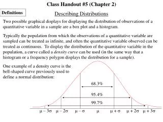
Class Handout #5 (Chapter 2) Definitions Describing Distributions Two possible graphical displays for displaying the distribution of observations of a quantitative variable in a sample are a box plot and a histogram. Typically the population from which the observations of a quantitative variable are sampled can be treated as infinite, and often the quantitative variable observed can be treated as continuous. To display the distribution of the quantitative variable in the population, a curve called a density curve can be used (in the same way that a histogram or a frequency polygon displays the distribution for a sample). One example of a density curve is the bell-shaped curve previously used to define a normal distribution: 68.3% 95.4% 99.7% – 3 – 2 – + + 2 + 3
A few examples of some other types of density functions are as follows: continued next page
The following two characteristics about the shape of a distribution are often of interest: Skewness in a distribution refers to the type and amount of non-symmetry present in the distribution. A distribution is called positively skewed when larger values tend to be more dispersed (perhaps resulting in a few unusually high values) and called negatively skewed when smaller values tend to be more dispersed (perhaps resulting in a few unusually small values).
Kurtosis in a symmetric (at least approximately) distribution refers to the proportion (or probability) of values more than one standard deviation away from the mean (in either direction). A symmetric distribution where the proportion (or probability) of values more than one standard deviation away from the mean is lower than that for a normal distribution is called platykurtic. A symmetric distribution where the proportion (or probability) of values more than one standard deviation away from the mean is higher than that for a normal distribution is called leptokurtic. mean– median ————–—–—– standard deviation The skewness ratio is from the work of Pearson, Stuart, and Ord. In practice, the measure of skewness usually used and usually available from statistical software, such as SPSS, is the Fisher skewness coefficient, which is based on the third power of deviations from the mean. The measure of kurtosis usually used and usually available from statistical software, such as SPSS, is the Fisher kurtosis coefficient. For SPSS data, each of these two Fisher coefficients are available together with a standard error. For data selected from a normal distribution, it is expected that each coefficient does not differ by more than two standard errors away from zero; one or both coefficients being more than two standard errors away from zero in either direction is an indication that the data comes from some non-normal distribution.
1. Displayed below are several histograms, each representing a possible distribution of a sample of observations of a quantitative variable. Uniform Distribution Bell-Shaped Distribution Positively Skewed Distribution Negatively Skewed Distribution Bimodal U-Shaped Distribution
1. - continued Indicate which histogram would correspond to each box plot displayed below. Uniform Distribution Bell-Shaped Distribution Positively Skewed Distribution Negatively Skewed Distribution Bimodal U-Shaped Distribution
2. For each characteristic listed, indicate which histogram(s) displayed in #1 represent data that would satisfy the characteristic. the distribution is symmetric (a) (b) (c) (d) (e) (f) Bimodal U-Shaped Distribution Uniform Distribution Bell-Shaped Distribution the mean is larger than the median Positively Skewed Distribution the mean is smaller than the median Negatively Skewed Distribution the mean and the median are equal or very close in value Bimodal U-Shaped Distribution Uniform Distribution Bell-Shaped Distribution more than half of the values are above the mean Negatively Skewed Distribution more than half of the values are below the mean Positively Skewed Distribution 3. For each hypothesis test listed in the tables titled and , indicate what assumptions the data are required to satisfy, in order to complete the tables.
Hypothesis Tests Involving One Variable random sample from a normal distribution OR from a non-normal distribution with “sufficiently large” sample size random sample of quantitative or qualitative-ordinal observations from a symmetric distribution random sample of qualitative observations with a sample size large enough so that each expected frequency is at least 5 Hypothesis Tests Involving Two Variables random sample of differences from a normal distribution OR from a non-normal distribution with “sufficiently large” sample size
two independent random samples from distributions having equal variance where each distribution is normal OR from non-normal distributions with “sufficiently large” sample sizes two independent random samples from respective normal distributions OR from non-normal distributions with “sufficiently large” sample sizes independent random samples from distributions having equal variance where each distribution is normal OR from non-normal distributions with “sufficiently large” sample sizes randomly selected observations for a contingency table with two qualitative variables where each expected frequency is at least 5 when assuming independence Return to the beginning of the handout:
Many commonly used inferential statistical procedures are based on the assumption that a random sample of data comes from a normal distribution. If there is concern that this assumption is not satisfied and that a statistical procedure based on this assumption might not be appropriate, data transformation can be used to produce a distribution that is at least approximately a normal distribution without affecting the original meaning of the data. Such data transformations can also be used when other assumptions (such as equal variance, linearity) are violated. The Shapiro-Wilk test is often used to decide if there is sufficient evidence that a random sample of data is from a non-normal distribution. With SPSS, Shapiro-Wilk test results can be obtained for each variable in an SPSS data file; these test results are accompanied by a normal probability plot, which is a scatter plot where the axes are scaled so that the points will be closer to lying on a diagonal straight line as the data looks more like it came from a normal distribution. It has been recommended that non-normality need not be considered a serious problem unless extreme skewness or extreme departure from normality with regard to kurtosis is observed in descriptive statistics (i.e., a coefficient more than three standard errors away from zero) or graphical displays, or unless p < 0.001 in the Shapiro-Wilk test. With a small sample size, say less than 10, it can be difficult to detect non-normality in a distribution. Consequently, with small sample sizes, unless there is a high degree of certainty that a population has a normal distribution, it is wise to employ procedures that do not require normality at least as a verification of results.
4. The SPSS data file ceo contains the ages (in years) and the yearly salaries ($1000s) of the chief executive officer (CEO) for 20 small firms in 1993, and this data was treated as a random sample in Exercises #6 and #8 of Class Handout #3, where statistical analyses based on the assumption of random selection from a normal distribution was performed. (a) With this data and the appropriate guidelines in the document titled Using SPSS Version 19.0, use SPSS to obtain statistics and create graphs in order to check for normality and skewness in the variables age and yearly salary.
4. - continued (b) For each of the variables age and salary, compare the skewnessand kurtosis coefficients to their respective standard errors (from the SPSS output in part (a)), look at the results of the Shapiro-Wilk test, and complete the corresponding statement about whether or not non-normality needs to be a concern with regard to statistical analysis. For the variable age in the data, the skewness coefficient (______ with s.e. = ______) and the kurtosis coefficient (______ with s.e. = ______) are each less than one standard error away from zero; also, p = ______ is not less than 0.001 in the Shapiro-Wilk test. Consequently, non-normality is _______________________________ _____________________________________________ _____________________________________________ 0.512 0.466 0.670 0.992 0.798 not a concern with regard to statistical analysis involving the variable age.
For the variable salary in the data, the skewness coefficient (______ with s.e. = ______) and the kurtosis coefficient (______ with s.e. = ______) are each less than one standard error away from zero; also, p = ______ is not less than 0.001 in the Shapiro-Wilk test. Consequently, non-normality is ____________________ _____________________________________________ _____________________________________________ 0.512 0.388 0.575 0.992 0.348 not a concern with regard to statistical analysis involving the variable salary. (c) Based on the conclusions in part (b), what can we say about the statistical analyses in Exercises #6 and #8 of Class Handout #3, based on the assumption of random selection from a normal distribution? We can say that the assumption of selection from a normal distribution can be considered satisfied for the statistical analyses in Exercises #6 and #8 of Class Handout #3.
5. The SPSS data file metabolismcontains the measurements of body temperature in degrees Fahrenheit and heart rate in beats per minute for a sample of males and for a sample of females, and we shall treat the data for each sex as a random sample, which was done for males in Exercise #9 of Class Handout #3, where statistical analysis based on the assumption of random selection from a normal distribution was performed. Use this data in SPSS to do the following: (a) With this data and the appropriate guidelines in the document titled Using SPSS Version 19.0, use SPSS to obtain statistics and create graphs in order to check for normality and skewness in the variables body temperatureand heart rate for each sex.
(b) For each of the sexes with the variable body temperature, compare the skewnessand kurtosis coefficients to their respective standard errors (from the SPSS output in part (a)), look at the results of the Shapiro-Wilk test, and complete the corresponding statement about whether or not non-normality needs to be a concern with regard to statistical analysis. For the variable body temperature among the males in the data, the skewness coefficient (______ with s.e. = ______) and the kurtosis coefficient (______ with s.e. = ______) are each less than one standard error away from zero; also, p = ______ is not less than 0.001 in the Shapiro-Wilk test. Consequently, non-normality is _____________________________________________ _____________________________________________ 0.213 0.297 0.371 0.586 0.855 not a concern with regard to statistical analysis involving the variable body temperature among males.
5. - continued For the variable body temperature among the females in the data, the skewness coefficient (______ with s.e. = ______) is less than one standard error away from zero, and the kurtosis coefficient (______ with s.e. = ______) is almost three standard errors away from zero; also, although there are a few outliers in the distribution, p= ______ is not less than 0.001 in the Shapiro-Wilk test. Consequently, non-normality is ___________________ _____________________________________________ _____________________________________________ 0.098 0.297 1.685 0.586 0.090 not a concern with regard to statistical analysis involving the variable body temperature among females.
(c) For each of the sexes with the variable heart rate, compare the skewnessand kurtosis coefficients to their respective standard errors (from the SPSS output in part (a)), look at the results of the Shapiro-Wilk test, and complete the corresponding statement about whether or not non-normality needs to be a concern with regard to statistical analysis. For the variable heart rate among the males in the data, the skewness coefficient (______ with s.e. = ______) and the kurtosis coefficient (______ with s.e. = ______) are each less than one standard error away from zero; also, p = ______ is not less than 0.001 in the Shapiro-Wilk test. Consequently, non-normality is _____________________________________________ _____________________________________________ 0.051 0.297 0.321 0.586 0.791 not a concern with regard to statistical analysis involving the variable heart rate among males.
5. - continued For the variable heart rate among the females in the data, the skewness coefficient (______ with s.e. = ______) and the kurtosis coefficient (______ with s.e. = ______) are each less than two standard errors away from zero; also, p = ______ is not less than 0.001 in the Shapiro-Wilk test. Consequently, non-normality is _____________________________________________ _____________________________________________ 0.293 0.297 0.717 0.586 0.148 not a concern with regard to statistical analysis involving the variable heart rate among females.
(d) Based on the conclusion for males in part (c), what can we say about the statistical analyses in Exercise #9 of Class Handout #3, based on the assumption of random selection from a normal distribution? We can say that the assumption of selection from a normal distribution can be considered satisfied for the statistical analyses in Exercise #9 of Class Handout #3. Next class, we shall consider Exercise #6, which involves an additional step not in either of the two previous exercises.