Download
1 / 12
120 likes | 243 Views
Explore the innovative computer-intensive method of bootstrapping, essential for data analysis in industrial statistics. This course, led by Dr. Ron S. Kenett, covers foundational concepts such as variability, sampling for estimation, parametric statistical inference, and multiple linear regression, all framed within the context of bootstrapping. Learn to derive empirical bootstrap distributions, estimate confidence intervals, and apply these techniques to real-world scenarios. Resources include the textbook "Modern Industrial Statistics" by Kenett and Zacks. ###

E N D
Computer Intensive Techniques (Bootstrapping) Instructor: Ron S. Kenett Email: ron@kpa.co.il Course Website: www.kpa.co.il/biostat Course textbook: MODERN INDUSTRIAL STATISTICS, Kenett and Zacks, Duxbury Press, 1998 (c) 2000, Ron S. Kenett, Ph.D.
Course Syllabus • Understanding Variability • Variability in Several Dimensions • Basic Models of Probability • Sampling for Estimation of Population Quantities • Parametric Statistical Inference • Computer Intensive Techniques • Multiple Linear Regression • Statistical Process Control • Design of Experiments (c) 2000, Ron S. Kenett, Ph.D.
Bootstrapping A computer intensive method, introduced in 1979 by Brad Efron from Stanford University in order to “pool yourself out of the mess”: • Take a Random Sampling With Replacement (RSWR) and compute statistic T • Resample M times and recompute statistic T • Derive Empirical Bootstrap Distribution (EBD) • E{EBD} and STD{EBD} and EBD percentiles estimate E{T} and STD{T} and Bootstrap Confidence Interval for population parameter (c) 2000, Ron S. Kenett, Ph.D.
Bootstrap testing of the mean Hybrid1 2060 2127 1947 2140 1960 1960 2134 2054 2094 2087 2267 2427 2174 2107 2267 2154 2167 2147 2214 2160 2180 2220 2167 2174 2280 2187 2180 2060 2060 2054 2240 2140 Is this significantly different from 2150 ? (c) 2000, Ron S. Kenett, Ph.D.
Boot1smp.exe (c) 2000, Ron S. Kenett, Ph.D.
Hybrid1 2060 2127 1947 2140 1960 1960 2134 2054 2094 2087 2267 2427 2174 2107 2267 2154 2167 2147 2214 2160 2180 2220 2167 2174 2280 2187 2180 2060 2060 2054 2240 2140 Hybrid1 2060 2127 1947 2140 1960 1960 2134 2054 2094 2087 2267 2427 2174 2107 2267 2154 2167 2147 2214 2160 2180 2220 2167 2174 2280 2187 2180 2060 2060 2054 2240 2140 Hybrid1 2060 2127 1947 2140 1960 1960 2134 2054 2094 2087 2267 2427 2174 2107 2267 2154 2167 2147 2214 2160 2180 2220 2167 2174 2280 2187 2180 2060 2060 2054 2240 2140 Hybrid1 2060 2127 1947 2140 1960 1960 2134 2054 2094 2087 2267 2427 2174 2107 2267 2154 2167 2147 2214 2160 2180 2220 2167 2174 2280 2187 2180 2060 2060 2054 2240 2140 Hybrid1 2060 2127 1947 2140 1960 1960 2134 2054 2094 2087 2267 2427 2174 2107 2267 2154 2167 2147 2214 2160 2180 2220 2167 2174 2280 2187 2180 2060 2060 2054 2240 2140 RSWR (c) 2000, Ron S. Kenett, Ph.D.
Empirical Bootstrap Distribution *Derive reference distribution by computing X-bar Std 2135.03 87.850 2149.84 121.631 2141.19 109.258 2149.09 78.084 2134.00 103.856 2122.13 73.843 2119.66 86.625 2113.59 107.136 2138.97 101.693 2163.00 67.725 (c) 2000, Ron S. Kenett, Ph.D.
Empirical Bootstrap Distribution Empirical Bootstrap Distribution of mean 0.95 conf. BI = (2109.5, 2179.9) EBD of STD 2150 (c) 2000, Ron S. Kenett, Ph.D.
Bootstrapping the ANOVA Hybrid1 Hybrid2 Hybrid3 2060 1907 1887 2127 1940 1834 1947 1700 1587 2140 1934 1814 1960 1707 1614 1960 1680 1680 2134 1940 1747 2054 1794 1660 2094 1707 1600 F= MSBetween/MSWithin = 49.274 (c) 2000, Ron S. Kenett, Ph.D.
EBD of F values ANOVTEST.EXE F= 49.274 (c) 2000, Ron S. Kenett, Ph.D.
Bootstrapping Stress Strength relationships • Draw samples from X and Y • X: Stress or Load distributions • Y: Strength distribution • Estimate P( X>Y) (c) 2000, Ron S. Kenett, Ph.D.
EBD of P(X>Y) • X= .0352, .0397, .0677, .0233, .0873, .1156, .0286, .0200, .0797, .9972, .0245, .0251, .0469, .0838, .0796 • Y= 1.7700, .9457, 1.8985, 2.6121, 1.0929, .0362, 1.0615, 2.3895, .0982, .7971, .8316, 3.2304, .4373, 2.5648, .6377 • P( X>Y) = 0.04 with P.95 = 0.08 (c) 2000, Ron S. Kenett, Ph.D.