Lecture 7 – Axial flow turbines

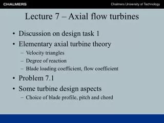
1. Lecture 7 – Axial flow turbines • Elementary axial turbine theory • Velocity triangles • Degree of reaction • Blade loading coefficient, flow coefficient • Problem 7.1 • Civil jet aircraft performance

2. Axial flow turbines • Working fluid is accelerated by the stator and decelerated by the rotor • Expansion occurs in stator and in relative frame of rotor • Boundary layer growth and separation does not limit stage loading as in axial compressor

3. Elementary theory • Energy equation for control volumes (again): • Adiabatic expansion process (work extracted from system - sign convention for added work = +w) • Rotor => -w = cp(T03-T02) <=> w = cp(T02-T03) • Stator => 0 = cp(T02-T01) => T02= T01

4. How is the temperature drop related to the blade angles ? • We study change of angular momentum at mid of blade (as approximation)

5. Governing equations and assumptions • Relative and absolute refererence frames are related by: • We only study designs where: • Ca2=Ca3 • C1=C3 • We repeat the derivation of theoretical work used for radial and axial compressors:

6. Principle of angular momentum Stage work output w: Ca constant:

7. (1)+(2) => (1) (2)

8. Combine derived equations => Energy equation Energy equation: We have a relation between temperature drop and blade angles!!! : Exercise: derive the correct expression when 3 is small enough to allow 3 to be pointing in the direction of rotation.

9. Dimensionless parameters Blade loading coefficient Degree of reaction Exercise: show that this expression is equal to => when C3= C1

10.  can be related to the blade angles! C3 = C1 => Relative to the rotor the flow does no work (in the relative frame the blade is fixed). Thus T0,relative is constant => Exercise: Verify this by using the definition of the relative total temperature:

11.  can be related to the blade angles! Plugging in results in definition of  => The parameter  quantifies relative amount of ”expansion” in rotor. Thus, equation 7.7 relates blade angles to the relative amount of expansion. Aircraft turbine designs are typically 50% degree of reaction designs.

12. Dimensionless parameters Finally, the flow coefficient: Current aircraft practice (according to C.R.S): Aircraft practice => relatively high values on flow and stage loading coefficients limit efficiencies

13. Dimensionless parameters Using the flow coefficient in 7.6 and 7.7 we obtain: The above equations and 7.1 can be used to obtain the gas and blade angles as a function of the dimensionless parameters

14. Two suggested exercises • Exercise: show that the velocity triangles become symmetric for = 0.5. Hint combine 7.1 and 7.9 • Exercise: use the “current aircraft practice” rules to derive bounds for what would be considered conventional aircraft turbine designs. What will be the range for 3? Assume = 0.5.

15. Turbine loss coefficients: Nozzle (stator) loss coefficients: Nozzle (rotor) loss coefficients:

16. Problem 7.1

17. Civil jet aircraft performance

18. Resulting force perpendicular to the flight path Four forces of flight Net thrust from the engines α angle of attack V velocity Newton’s second law resulting force parallell to the flight path

19. L=Lift = q·S·CL [N] D=Drag = q·S·CD[N] q = dynamic pressure [N/m²] S = reference wing area [m²] CL= coefficient of lift CL=f(α,Re,M) CD= coefficient of drag CD = f(α,Re,M) Aerodynamic equations

20. Reference wing area The area is considered to extend without interruption through the fuselage and is usually denoted S.

21. Lift versus angle of attack

23. The ISA Atmosphere From lecture 5

24. Equations

25. Lift equation

26. Drag equation

27. Drag polar

28. High speed drag polar

29. Taxi Take off Climb Cruise Descent Approach and landing Diversion to alternate airport? A flight consists of:

30. Cruise For an airplane to be in level, unaccelerated flight, thrust and drag must be equal and opposite, and the lift and weight must be equal and opposite according to the laws of motion, i.e. Lift = Weight = mg Thrust = Drag

31. Range

32. Range

33. Breguet range equation For a preliminary performance analysis is the range equation usually simplified. If we assume flight at constant altitude, M, SFC and L/D the range equation becomes which is frequently called the Breguet range equation

34. Breguet range equation The Breuget range equation is written directly in terms of SFC. Clearly maximum range for a jetaircraft is not dictated by maximum L/D, but rather the maximum value of the product M(L/D) or V(L/D).

35. Breuget range equation From the simplified range equation, maximum range is obtained from • Flight at maximum • Low SFC • High altitude, low ρ • Carrying a lot of fuel

36. Range

37. Endurance Endurance is the amout of time that an aircraft can stay in the air on one given load of fuel

38. Endurance

39. Learning goals • Understand how turbine blade angles relate to work output • Be familiar with the three non-dimensional parameters: • Blade loading coefficient, degree of reaction, flow coefficient • Understand why civil aircraft are • operated at high altitude • at flight Mach numbers less than 1.0 • How engine performance influences aircraft range