Part II: Concurrency Control
440 likes | 494 Views
Learn about the theoretical foundations and practical implications of concurrency control in transactional information systems. Explore various correctness notions, synchronization problems, and serialization concepts.

Part II: Concurrency Control
E N D
Presentation Transcript
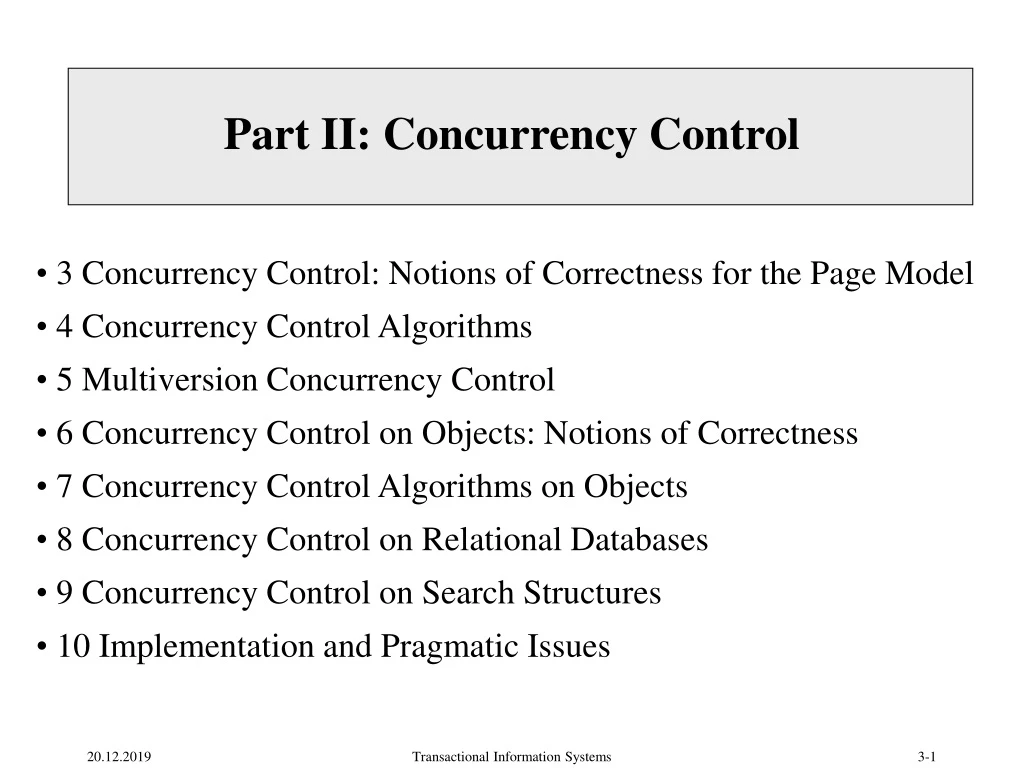
Part II: Concurrency Control • 3 Concurrency Control: Notions of Correctness for the Page Model • 4 Concurrency Control Algorithms • 5 Multiversion Concurrency Control • 6 Concurrency Control on Objects: Notions of Correctness • 7 Concurrency Control Algorithms on Objects • 8 Concurrency Control on Relational Databases • 9 Concurrency Control on Search Structures • 10 Implementation and Pragmatic Issues Transactional Information Systems
Chapter 3: Concurrency Control – Notions of Correctness for the Page Model • 3.2 Canonical Synchronization Problems • 3.3 Syntax of Histories and Schedules • 3.4 Correctness of Histories and Schedules • 3.5 Herbrand Semantics of Schedules • 3.6 Final-State Serializability • 3.7 View Serializability • 3.8 Conflict Serializability • 3.9 Commit Serializability • 3.10 An Alternative Criterion: Interleaving Specifications • 3.11 Lessons Learned „Nothing is as practical as a good theory“ (Albert Einstein) Transactional Information Systems
Lost Update Problem P1 Time P2 /* x = 100 */ r (x) 1 2 r (x) x := x+1004 x := x+200 w (x) 5 /* x = 200 */ 6 w (x) /* x = 300 */ update „lost“ Observation: problem is the interleaving r1(x) r2(x) w1(x) w2(x) Transactional Information Systems
Inconsistent Read Problem P1 Time P2 1 r (x) 2 x := x – 10 3 w (x) sum := 0 4 r (x) 5 r (y) 6 sum := sum +x 7 sum := sum + y 8 9 r (y) 10 y := y + 10 11 w (y) „sees“ wrong sum Observations: problem is the interleaving r2(x) w2(x) r1(x) r1(y) r2(y) w2(y) no problem with sequential execution Transactional Information Systems
Dirty Read Problem P1 Time P2 r (x) 1 x := x + 100 2 w (x) 3 4 r (x) 5 x := x - 100 failure & rollback 6 7 w (x) cannot rely on validity of previously read data Observation: transaction rollbacks could affect concurrent transactions Transactional Information Systems
Chapter 3: Concurrency Control – Notions of Correctness for the Page Model • 3.2 Canonical Synchronization Problems • 3.3 Syntax of Histories and Schedules • 3.4 Correctness of Histories and Schedules • 3.5 Herbrand Semantics of Schedules • 3.6 Final-State Serializability • 3.7 View Serializability • 3.8 Conflict Serializability • 3.9 Commit Serializability • 3.10 An Alternative Criterion: Interleaving Specifications • 3.11 Lessons Learned Transactional Information Systems
Schedules and Histories • Definition 3.4 (Schedules and histories): • Let T={t1, ..., tn} be a set of transactions, where each ti T • has the form ti=(opi, <i) with opi denoting the operations of ti • and <i their ordering. • A history for T is a pair s=(op(s),<s) s.t. • (a) op(s) i=1..n opi i=1..n {ai, ci} • (b) for all i, 1in: ci op(s) ai op(s) • (c) i=1..n <i <s • (d) for all i, 1in, and all p opi: p <s ci or p <s ai • (e) for all p, q op(s) s.t. at least one of them is a write • and both access the same data item: p <s q or q <s p • (ii) A schedule is a prefix of a history. Definition 3.5 (Serial history): A history s is serial if for any two transactions ti and tj in s, where ij, all operations from ti are ordered in s before all operations from tj or vice versa. Transactional Information Systems
r1(x) w1(x) c1 r1(z) r2(x) w2(y) c2 r3(z) w3(y) c3 w3(z) Example Schedules and Notation Example 3.6: trans(s):= {ti | s contains step of ti} commit(s):= {ti trans(s) | ci s} abort(s):= {ti trans(s) | ai s} active(s):= trans(s) – (commit(s) abort(s)) Example 3.8: r1(x) r2(z) r3(x) w2(x) w1(x) r3(y) r1(y) w1(y) w2(z) w3(z) c1 a3 Transactional Information Systems
Chapter 3: Concurrency Control – Notions of Correctness for the Page Model • 3.2 Canonical Synchronization Problems • 3.3 Syntax of Histories and Schedules • 3.4 Correctness of Histories and Schedules • 3.5 Herbrand Semantics of Schedules • 3.6 Final-State Serializability • 3.7 View Serializability • 3.8 Conflict Serializability • 3.9 Commit Serializability • 3.10 An Alternative Criterion: Interleaving Specifications • 3.11 Lessons Learned Transactional Information Systems
Correctness of Schedules • Define equivalence relation on set S of all schedules. • „Good“ schedules are those in the equivalence classes • of serial schedules. • Equivalence must be efficiently decidable. • „Good“ equivalence classes should be „sufficiently large“. Disregard aborts: assume that all transactions are committed. Transactional Information Systems
Chapter 3: Concurrency Control – Notions of Correctness for the Page Model • 3.2 Canonical Synchronization Problems • 3.3 Syntax of Histories and Schedules • 3.4 Correctness of Histories and Schedules • 3.5 Herbrand Semantics of Schedules • 3.6 Final-State Serializability • 3.7 View Serializability • 3.8 Conflict Serializability • 3.9 Commit Serializability • 3.10 An Alternative Criterion: Interleaving Specifications • 3.11 Lessons Learned Transactional Information Systems
Herbrand Semantics of Schedules • Definition 3.9 (Herbrand semantics of steps): • For schedule s the Herbrand semantics Hs of steps ri(x), wi(x) op(s) is: • Hs[ri(x)] := Hs[wj(x)] where wj(x) is the last write on x in s before ri(x). • Hs[wi(x)] := fix(Hs[ri(y1), ..., Hs[ri(ym)]) where • the ri(yj), 1jm, are all read operations of ti that occcur in s before wi(x) • and fix is an uninterpreted m-ary function symbol. • Definition 3.10 (Herbrand universe): • For data items D={x, y, z, ...} and transactions ti, 1in, the Herbrand universe • HU is the smallest set of symbols s.t. • f0x( ) HU for each x D where f0x is a constant, and • if wi(x) opi for some ti, there are m read operations ri(y1), ..., ri(ym) • that precede wi(x) in ti, and v1, ..., vm HU, then fix (v1, ..., vm) HU. Definition 3.11 (Schedule semantics): The Herbrand semantics of a schedule s is the mapping H[s]: D HU defined by H[s](x) := Hs[wi(x)], where wi(x) is the last operation from s writing x, for each x D. Transactional Information Systems
Herbrand Semantics: Example s = w0(x) w0(y) c0 r1(x) r2(y) w2(x) w1(y) c2 c1 Hs[w0(x)] = f0x( ) Hs[w0(y)] = f0y( ) Hs[r1(x)] = Hs[w0(x)] = f0x( ) Hs[r2(y)] = Hs[w0(y)] = f0y( ) Hs[w2(x)] = f2x(Hs[r2(y)]) = f2x(f0y( )) Hs[w1(y)] = f1y(Hs[r1(x)]) = f1y(f0x( )) H[s](x) = Hs[w2(x)] = f2x(f0y( )) H[s](y) = Hs[w1(y)] = f1y(f0x( )) Transactional Information Systems
Chapter 3: Concurrency Control – Notions of Correctness for the Page Model • 3.2 Canonical Synchronization Problems • 3.3 Syntax of Histories and Schedules • 3.4 Correctness of Histories and Schedules • 3.5 Herbrand Semantics of Schedules • 3.6 Final-State Serializability • 3.7 View Serializability • 3.8 Conflict Serializability • 3.9 Commit Serializability • 3.10 An Alternative Criterion: Interleaving Specifications • 3.11 Lessons Learned Transactional Information Systems
Final-State Equivalence Definition 3.12 (Final-state equivalence): Schedules s and s‘ are called final-state equivalent, denoted s f s‘, if op(s)=op(s‘) and H[s]=H[s‘]. Example 1: s= r1(x) r2(y) w1(y) r3(z) w3(z) r2(x) w2(z) w1(x) s‘= r3(z) w3(z) r2(y) r2(x) w2(z) r1(x) w1(y) w1(x) H[s](x) = Hs[w1(x)] = f1x(f0x( )) = Hs‘[w1(x)] = H[s‘](x) H[s](y) = Hs[w1(y)] = f1y(f0x( )) = Hs‘[w1(y)] = H[s‘](y) H[s](z) = Hs[w2(z)] = f2z(f0x( ), f0y( )) = Hs‘[w2(z)] = H[s‘](z) s f s‘ Example 2: s= r1(x) r2(y) w1(y) w2(y) s‘= r1(x) w1(y) r2(y) w2(y) H[s](y) = Hs[w2(y)] = f2y(f0y( )) H[s‘](y) = Hs‘[w2(y)] = f2y(f1y(f0x( ))) (s f s‘) Transactional Information Systems
Reads-from Relation • Definition 3.13 (Reads-from relation; useful, alive, and dead steps): • Given a schedule s, extended with an initial and a final transaction, t0 and t. • rj(x)reads x in s from wi(x) if wi(x) is the last write on x s.t. wi(x) <s rj(x). • The reads-from relation of s is • RF(s) := {(ti, x, tj) | an rj(x) reads x from a wi(x)}. • (iii) Step p is directly useful for step q, denoted pq, if q reads from p, • or p is a read step and q is a subsequent write step of the same transaction. • *, the „useful“ relation, denotes the reflexive and transitive closure of . • Step p is alive in s if it is useful for some step from t, and dead otherwise. • The live-reads-from relation of s is • LRF(s) := {(ti, x, tj) | an alive rj(x) reads x from wi(x)} Example: s= r1(x) r2(y) w1(y) w2(y) s‘= r1(x) w1(y) r2(y) w2(y) RF(s) = {(t0,x,t1), (t0,y,t2), (t0,x,t), (t2,y,t)} RF(s‘) = {(t0,x,t1), (t1,y,t2), (t0,x,t), (t2,y,t)} LRF(s) = {(t0,y,t2), (t0,x,t), (t2,y,t)} LRF(s‘) = {(t0,x,t1), (t1,y,t2), (t0,x,t), (t2,y,t)} Transactional Information Systems
Final-State Serializability • Theorem 3.15: • For schedules s and s‘ the following statements hold. • s f s‘ iff op(s)=op(s‘) and LRF(s)=LRF(s‘). • For s let the step graph D(s)=(V,E) be a directed graph with vertices • V:=op(s) and edges E:={(p,q) | pq}, and the reduced step graph D1(s) be • derived from D(s) by removing all vertices that correspond to dead steps. • Then LRF(s)=LRF(s‘) iff D1(s)=D1(s‘). Corollary 3.18: Final-state equivalence of two schedules s and s‘ can be decided in time that is polynomial in the length of the two schedules. Definition 3.19 (Final-state serializability): A schedule s is final-state serializable if there is a serial schedule s‘ s.t. s f s‘. FSR denotes the class of all final-state serializable histories. Transactional Information Systems
FSR: Example s= r1(x) r2(y) w1(y) w2(y) s‘= r1(x) w1(y) r2(y) w2(y) D(s): D(s‘): w0(x) w0(y) w0(x) w0(y) r2(y) r1(x) w1(y) r1(x) w1(y) r2(y) w2(y) w2(y) r(x) r(y) r(x) r(y) dead steps Transactional Information Systems
Chapter 3: Concurrency Control – Notions of Correctness for the Page Model • 3.2 Canonical Synchronization Problems • 3.3 Syntax of Histories and Schedules • 3.4 Correctness of Histories and Schedules • 3.5 Herbrand Semantics of Schedules • 3.6 Final-State Serializability • 3.7 View Serializability • 3.8 Conflict Serializability • 3.9 Commit Serializability • 3.10 An Alternative Criterion: Interleaving Specifications • 3.11 Lessons Learned Transactional Information Systems
Canonical Anomalies Reconsidered • Lost update anomaly: • L = r1(x) r2(x) w1(x) w2(x) c1 c2 LRF(L) = {(t0,x,t2), (t2,x,t)} LRF(t1 t2) = {(t0,x,t1), (t1,x,t2), (t2,x,t)} LRF(t2 t1) = {(t0,x,t2), (t2,x,t1), (t1,x,t)} history is not FSR • Inconsistent read anomaly: • I = r2(x) w2(x) r1(x) r1(y) r2(y) w2(y) c1 c2 LRF(I) = {(t0,x,t2), (t0,y,t2), (t2,x,t,), (t2,x,t,)} LRF(t1 t2) = {(t0,x,t2), (t0,y,t2), (t2,x,t,), (t2,x,t,)} LRF(t2 t1) = {(t0,x,t2), (t0,y,t2), (t2,x,t,), (t2,x,t,)} • history is FSR ! Observation: (Herbrand) semantics of all read steps matters! Transactional Information Systems
View Serializability • Definition 3.24 (View equivalence): • Schedules s and s‘ are view equivalent, denoted s v s‘, if the following hold: • op(s)=op(s‘) • H[s] = H[s‘] • Hs[p] = Hs‘[p] for all (read or write) steps • Theorem 3.22: • For schedules s and s‘ the following statements hold. • s v s‘ iff op(s)=op(s‘) and RF(s)=RF(s‘) • s v s‘ iff D(s)=D(s‘) Corollary 3.23: View equivalence of two schedules s and s‘ can be decided in time that is polynomial in the length of the two schedules. Definition 3.24 (View serializability): A schedule s is view serializable if there exists a serial schedule s‘ s.t. s v s‘. VSR denotes the class of all view-serializable histories. Transactional Information Systems
Inconsistent Read Reconsidered • Inconsistent read anomaly: • I = r2(x) w2(x) r1(x) r1(y) r2(y) w2(y) c1 c2 • history is not VSR ! RF(I) = {(t0,x,t2), (t2,x,t1), (t0,y,t1), (t0,y,t2), (t2,x,t,), (t2,x,t,)} RF(t1 t2) = {(t0,x,t1), (t0,y,t1), (t0,x,t2), (t0,y,t2), (t2,x,t,), (t2,x,t,)} RF(t2 t1) = {(t0,x,t2), (t0,y,t2), (t2,x,t1), (t2,y,t1), (t2,x,t,), (t2,x,t,)} Observation: VSR properly captures our intuition Transactional Information Systems
Relationship Between VSR and FSR Theorem 3.25: VSR FSR. Theorem 3.26: Let s be a history without dead steps. Then s VSR iff s FSR. Transactional Information Systems
On the Complexity of Testing VSR Theorem 3.27: The problem of deciding for a given schedule s whether s VSR holds is NP-complete. Transactional Information Systems
Properties of VSR Let s be a schedule and T trans(s). T(s) denotes the projection of s onto T. A class E of histories is called monotone if the following holds: if s is in E, then T(s) is in E for each T trans(s). VSR is not monotone. Example: s = w1(x) w2(x) w2(y) c2 w1(y) c1 w3(x) w3(y) c3 {t1, t2}(s) = w1(x) w2(x) w2(y) c2 w1(y) c1 • VSR • VSR Transactional Information Systems
Chapter 3: Concurrency Control – Notions of Correctness for the Page Model • 3.2 Canonical Synchronization Problems • 3.3 Syntax of Histories and Schedules • 3.4 Correctness of Histories and Schedules • 3.5 Herbrand Semantics of Schedules • 3.6 Final-State Serializability • 3.7 View Serializability • 3.8 Conflict Serializability • 3.9 Commit Serializability • 3.10 An Alternative Criterion: Interleaving Specifications • 3.11 Lessons Learned Transactional Information Systems
Conflict Serializability • Definition 3.32 (Conflicts and conflict relations): • Let s be a schedule, t, t‘ trans(s), t t‘. • Two data operations p t and q t‘ are in conflict in s if • they access the same data item and at least one of them is a write. • {(p, q)} | p, q are in conflict and p <s q} is the conflict relation of s. Definition 3.33 (Conflict equivalence): Schedules s and s‘ are conflict equivalent, denoted s c s‘, if op(s) = op(s‘) and conf(s) = conf(s‘). Definition 3.34 (Conflict serializability): Schedule s is conflict serializable if there is a serial schedule s‘ s.t. s c s‘. CSR denotes the class of all conflict serializable schedules. Example 1: r1(x) r2(x) r1(z) w1(x) w2(y) r3(z) w3(y) c1 c2 w3(z) c3 Example 2: r2(x) w2(x) r1(x) r1(y) r2(y) w2(y) c1 c2 • CSR • CSR Transactional Information Systems
Properties of CSR Theorem 3.35: CSR VSR Example: s = w1(x) w2(x) w2(y) c2 w1(y) c1 w3(x) w3(y) c3 s VSR, but s CSR. Theorem 3.37: (i) CSR is monotone. (ii) s CSR T(s) VSR for all T trans(s) (i.e., CSR is the largest monotone subset of VSR). Transactional Information Systems
Conflict Graph Definition 3.38 (Conflict graph): Let s be a schedule. The conflict graph G(s) = (V, E) is a directed graph with vertices V := commit(s) and edges E := {(t, t‘) | t t and there are steps p t, q t‘ with (p, q) conf(s)}. Theorem 3.40: Let s be a schedule. Then s CSR iff G(s) is acyclic. Corollary 3.41: Testing if a schedule is in CSR can be done in time polynomial to the schedule‘s number of transactions. Example: s = r1(y) r3(w) r2(y) w1(y) w1(x) w2(x) w2(z) w3(x) c1 c3 c2 G(s): t2 t1 t3 Transactional Information Systems
Proof of the Conflict-Graph Theorem Proof of Theorem 3.40: (i) Let s be a schedule in CSR. So there is a serial schedule s‘ with conf(s) = conf(s‘). Now assume that G(s) has a cycle t1 t2 ... tk t1. This implies that there are pairs (p1, q2), (p2, q3), ... , (pk, q1) with pi ti, qi ti, pi <s q(i+1), and pi in conflict with q(i+1). Because s‘ c s, it also implies that pi <s‘ q(i+1). Because s‘ is serial, we obtain ti <s‘ t(i+1) for i=1, ..., k-1, and tk <s‘ t1. By transitivity we infer t1 <s‘ t2 and t2 <s‘ t1, which is impossible. This contradiction shows that the initial assumption is wrong. So G(s) is acyclic. (ii) Let G(s) be acyclic. So it must have at least one source node. The following topological sort produces a total order < of transactions: a) start with a source node (i.e., a node without incoming edges), b) remove this node and all its outgoing edges, c) iterate a) and b) until all nodes have been added to the sorted list. The total transaction ordering order < preserves the edges in G(s); therefore it yields a serial schedule s‘ for which s‘c s. Transactional Information Systems
Commutativity and Ordering Rules Commutativity rules: C1: ri(x) rj(y) ~ rj(y) ri(x) if ij C2: ri(x) wj(y) ~ wj(y) ri(x) if ij and xy C3: wi(x) wj(y) ~ wj(y) wi(x) if ij and xy Ordering rule: C4: oi(x), pj(y) unordered ~> oi(x) pj(y) if xy or both o and p are reads Example for transformations of schedules: s = w1(x) r2(x) w1(y) w1(z) r3(z) w2(y) w3(y) w3(z) ~>[C2] w1(x) w1(y) r2(x) w1(z) w2(y) r3(z) w3(y) w3(z) ~>[C2] w1(x) w1(y) w1(z) r2(x) w2(y) r3(z) w3(y) w3(z) = t1 t2 t3 Transactional Information Systems
Commutativity-based Reducibility Definition 3.43 (Commutativity-based equivalence): Schedules s and s‘ s.t. op(s)=op(s‘) are commutativity-based equivalent, denoted s ~* s‘, if s can be transformed into s‘ by applying rules C1, C2, C3, C4 finitely many times. Theorem 3.44: Let s and s‘ be schedules s.t. op(s)=op(s‘). Then s c s‘ iff s ~* s‘. Definition 3.45 (Commutativity-based reducibility): Schedule s is commutativity-based reducible if there is a serial schedule s‘ s.t. s ~* s‘. Corollary 3.46: Schedule s is commutativity-based reducible iff s CSR. Transactional Information Systems
Order Preserving Conflict Serializability Definition 3.48 (Order preservation): Schedule s is order-preserving conflict serializable if it is conflict equivalent to a serial schedule s‘ and for all t, t‘ trans(s): if t completely precedes t‘ in s, then the same holds in s‘. OCSR denotes the class of all schedules with this property. Theorem 3.49: OCSR CSR. Example: s = w1(x) r2(x) c2 w3(y) c3 w1(y) c1 • CSR • OCSR Transactional Information Systems
Commit-order Preserving Conflict Serializability Definition 3.50 (Commit-order preservation): Schedule s is commit-order-preserving conflict serializable if for all ti, tj trans(s): if there are p ti, q tj with (p,q) conf(s) then ci <s cj. COCSR denotes the class of all schedules with this property. Theorem 3.51: COCSR CSR. Theorem 3.52: Schedule s is in COCSR iff there is a serial schedule s‘ s.t. s c s‘ and for all ti, tj trans(s): ti <s‘ tj ci <s cj. Theorem 3.53: COCSR OCSR. Example: s = w3(y) c3 w1(x) r2(x) c2 w1(y) c1 • OCSR • COCSR Transactional Information Systems
Chapter 3: Concurrency Control – Notions of Correctness for the Page Model • 3.2 Canonical Synchronization Problems • 3.3 Syntax of Histories and Schedules • 3.4 Correctness of Histories and Schedules • 3.5 Herbrand Semantics of Schedules • 3.6 Final-State Serializability • 3.7 View Serializability • 3.8 Conflict Serializability • 3.9 Commit Serializability • 3.10 An Alternative Criterion: Interleaving Specifications • 3.11 Lessons Learned Transactional Information Systems
Commit Serializability Definition 3.54 (Closure properties of schedule classes): Let E be a class of schedules. For schedule s let CP(s) denote the projection commit(s) (s). E is prefix-closed if the following holds: s E p E for each prefix of s. E is commit-closed if the following holds: s E CP(s) E. Theorem 3.55: CSR is prefix-commit-closed, i.e., prefix-closed and commit-closed. Definition 3.56 (Commit serializability): Schedule s is commit--serializable if CP(p) is -serializable for each prefix p of s, where can be FSR, VSR, or CSR. The resulting classes of commit--serializable schedules are denoted CMFSR, CMVSR, and CMCSR. Theorem 3.57: (i) CMFSR, CMVSR, CMCSR are prefix-commit-closed. (ii) CMCSR CMVSR CMFSR Transactional Information Systems
Chapter 3: Concurrency Control – Notions of Correctness for the Page Model • 3.2 Canonical Synchronization Problems • 3.3 Syntax of Histories and Schedules • 3.4 Correctness of Histories and Schedules • 3.5 Herbrand Semantics of Schedules • 3.6 Final-State Serializability • 3.7 View Serializability • 3.8 Conflict Serializability • 3.9 Commit Serializability • 3.10 An Alternative Criterion: Interleaving Specifications • 3.11 Lessons Learned Transactional Information Systems
Interleaving Specifications: Motivation Example: all transactions known in advance transfer transactions on checking accounts a and b and savings account c: t1 = r1(a) w1(a) r1(c) w1(c) t2 = r2(b) w2(b) r2(c) w2(c) balance transaction: t3 = r3(a) r3(b) r3(c) audit transaction: t4 = r4(a) r4(b) r4(c) w4(z) Possible schedules: r1(a) w1(a) r2(b) w2(b) r2(c) w2(c) r1(c) w1(c) r1(a) w1(a) r3(a) r3(b) r3(c) r1(c) w1(c) r1(a) w1(a) r2(b) w2(b) r1(c) r2(c) w2(c) w1(c) r1(a) w1(a) r4(a) r4(b) r4(c) w4(z) r1(c) w1(c) • CSR application-tolerable interleavings • CSR • CSR non-admissable interleavings • CSR Observations: application may tolerate non-CSR schedules a priori knowledge of all transactions impractical Transactional Information Systems
Indivisible Units Definition 3.58 (Indivisible units): Let T={t1, ..., tn} be a set of transactions. For ti, tj T, titj, an indivisible unit of ti relative to tj is a sequence of consecutive steps of ti s.t. no operations of tj are allowed to interleave with this sequence. IU(ti, tj) denotes the ordered sequence of indivisible units of ti relative to tj. IUk(ti, tj) denotes the kth element of IU(ti, tj). Example 3.59: t1 = r1(x) w1(x) w1(z) r1(y) t2 = r2(y) w2(y) r2(x) t3 = w3(x) w3(y) w3(z) IU(t1, t2) = < [r1(x) w1(x)], [w1(z) r1(y)] > IU(t1, t3) = < [r1(x) w1(x)], [w1(z)], [r1(y)] > IU(t2, t1) = < [r2(y)], [w2(y) r2(x)] > IU(t2, t3) = < [r2(y) w2(y)], [r2(x)] > IU(t3, t1) = < [w3(x) w3(y)], [w3(z)] > IU(t3, t2) = < [w3(x) w3(y)], [w3(z)] > s1 = r2(y) r1(x) w1(x) w2(y) r2(x) w1(z) w3(x) w3(y) r1(y) w3(z) • respects all IUs s2 = r1(x) r2(y) w2(y) w1(x) r2(x) w1(z) r1(y) • violates IU1(t1, t2) and IU2(t2, t1) but is conflict equivalent to an allowed schedule Transactional Information Systems
Relatively Serializable Schedules Definition 3.61 (Dependence of steps): Step q directly depends on step p in schedule s, denoted p~>q, if p <s q and either p, q belong to the same transaction t and p <t q or p and q are in conflict. ~>* denotes the reflexive and transitive closure of ~>. Definition 3.62 (Relatively serial schedule): s is relatively serial if for all transactions ti, tj: if q tj is interleaved with some IUk(ti, tj), then there is no operation p IUk(ti, tj) s.t. p~>* q or q~>* p Example 3.63: s4 = r1(x) r2(y) w1(x) w2(y) w3(x) w1(z) w3(y) r2(x) r1(y) w3(z) Definition 3.64 (Relatively serializable schedule): s is relatively serializable if it is conflict equivalent to a relatively serial schedule. Example 3.65: s4 = r1(x) r2(y) w2(y) w1(x) w3(x) r2(x) w1(z) w3(y) r1(y) w3(z) Transactional Information Systems
Relative Serialization Graph • Definition 3.67 (Push forward and pull backward): • Let IUk(ti, tj) be an IU of ti relative to tj. For an operation pi IUk(ti, tj) let • F(pi, tj) be the last operation in IUk(ti, tj) and • B(pi, tj) be the first operation in IUk(ti, tj). • Definition 3.68 (Relative serialization graph): • The relative serialization graph RSG(s) = (V,E) of schedule s is a graph • with vertices V := op(s) and edge set E VV containing four types of edges: • for consecutive operations p, q of the same transaction (p, q) E (I-edge) • if p ~>* q for p ti, q tj, titj, then (p, q) E (D-edge) • if (p, q) is a D-edge with p ti, q tj, then (F(p, tj), q) E (F-edge) • if (p,q ) is a D-edge with p ti, q tj, then (p, B(q, ti)) E (B-edge) Theorem 3.71: A schedule s is relatively serializable iff RSG(s) is acyclic. Transactional Information Systems
RSG Example IU(t1, t2) = < [w1(x) r1(z)] > IU(t1, t3) = < [w1(x)], [r1(z)] > IU(t2, t1) = < [r2(x)], [w2(y)] > IU(t2, t3) = < [r2(x)], [w2(y)] > IU(t3, t1) = < [r3(z)], [r3(y)] > IU(t3, t2) = < [r3(z) r3(y)] > Example 3.69: t1 = w1(x) r1(z) t2 = r2(x) w2(y) t3 = r3(z) r3(y) s5 = w1(x) r2(x) r3(z) w2(y) r3(y) r1(z) RSG(s5): I w1(x) r1(z) D,B F D,B F I r2(x) w2(y) D,F,B B D,F B D,F I r3(z) r3(y) Transactional Information Systems
Chapter 3: Concurrency Control – Notions of Correctness for the Page Model • 3.2 Canonical Synchronization Problems • 3.3 Syntax of Histories and Schedules • 3.4 Correctness of Histories and Schedules • 3.5 Herbrand Semantics of Schedules • 3.6 Final-State Serializability • 3.7 View Serializability • 3.8 Conflict Serializability • 3.9 Commit Serializability • 3.10 An Alternative Criterion: Interleaving Specifications • 3.11 Lessons Learned Transactional Information Systems
Lessons Learned • Equivalence to serial history is a natural correctness criterion • CSR, albeit less general than VSR, • is most appropriate for • complexity reasons • its monotonicity property • its generalizability to semantically rich operations • OCSR and COCSR have additional beneficial properties Transactional Information Systems