
Chapter 5 MATRIX ALGEBRA: DETEMINANT, REVERSE, EIGENVALUES
E N D
Presentation Transcript
5.1 The Determinant of a Matrix • The determinant of a matrix is a fundamental concept of linear algebra that provides existence and uniqueness results for linear systems of equations; det A = |A| • LU factorization: A = LU, the determinant is |A| = |L||U| (5.1) • Doolittle method: L = lower triangular matrix with lii = 1 |L| = 1 |A| = |U| = u11u22…unn • Pivoting: each time we apply pivoting we need to change the sign of the determinant |A| = (-1)mu11u22…unn • Gauss forward elimination with pivoting:
Procedure for finding the determinant following the elimination method
The properties of the determinant • If A = BC |A| = |B||C| (A, B, C – square matrices) • |AT| = |A| • If two rows (or columns) are proportional, |A| = 0 • The determinant of a triangular matrix equals the product of its diagonal elements • A factor of any row (or column) can be placed before the determinant • Interchanging two rows (or columns) changes the determinant sign
5.2 Inverse of a Matrix • Definition: A-1 is the inverse of the square matrix A, if (5.5) I – identity matrix • A-1 = X (denote) AX = I (5.6) • LU factorization, Doolittle method: A = LU LY = I , UX = Y (5.7) • Here Y = {yij}, LY = I – lower triangular matrix with unity diagonal elements, i = 1,2,…,n; so for j from 1 to n • Also, X = {xij} vector, i = 1,2,…,n
Procedure for finding the inverse matrix following the LU factorization method
If Ax = b x = A-1b (A - matrix nxn, b, x – n-dimensional vectors) • If AX = B X = A-1B (A – matrix nxn, B,X – matrices nxm) – more often case. • We can write down this system as Axi = bi (i = 1,2,…,m) • xi, bi – vectors, ith rows of matrices X, B, respectively
X = A-1B calculating procedure following the method of LU factorization
5.3 Eigenvalues and Eigenvectors • Definition: let A be an nxn matrix • For some nonzero column vector x it may happen, for some scalar λ Ax = λx (5.9) • Then λ is an eigenvalue of A, x is eigenvector of A, associated with the eigenvalue λ; the problem of finding eigenvalue or eigenvector – eigen problem • Eq.(5.9) can be written in the form Av = λIv or (A – λI)x = 0 • If A is nonsingular matrix inverse exists det A ≠ 0 x = (A – λI)-10 = 0 • Hence, not to get zero solution x = 0, (A – λI) must not be nonsingular, i.e. det A = 0: (5.10) (5.11)
Eq. (5.11) -nth order algebraic equation with n unknowns (algebraic as well as complex) • Applying some numerical calculation, we can find λ • But when n is big, expanding to Eq.(5.11) is not the easy way to solve this method is not used much • Here: Jacobi and QR methods for finding eigenvalues
5.3.1 Jacobi method • Jacobi method is the direct method for finding eigenvalues and eigenvectors in case when A is the symmetric matrix • diag(a11,a12,…,ann) – diagonal matrix A • ei – unit vector with ith element = 1 and all others = 0 • The properties of egenvalues and eigenvectors: • if x – eigenvector of A, then ax is also eigenvector (a = constant) • if A – diagonal matrix, then aii are eigenvalues, ei is eigenvector • if R, Q are orthogonal matrices, then RQ is orthogonal • if λ – eigenvalue of A, x – eigenvector of A, R – orthogonal matrix, then λ is eigenvalue of RTAR, RTx is its eigenvector. RTAR is called similarity transformation • Eigenvalues of a symmetric matrix are real number
Jacobi method uses the properties mentioned above • A – arbitrary matrix, Ri – orthogonal matrix, RiTARi – similarity transformation (5.12) • - diagonal matrix following the 2nd property, the eigenvector is ei • We can write the eq.(5.12) as • Following the 3rd property, R1R2…Rn is orthogonal matrix; the 4th property – it has the same eigenvalues as A • The eigenvector of A is • Then the matrix consisting of xi as columns • Having found X, we find eigenvetors xi
Let’s consider 2-dimensional matrix example • The orthogonal matrix is • C, S – notation for cosθ, sinθ respectively • We need to choose θ so that the above matrix becomes diagonal • If a11≠a22, then • If a11=a22, then θ=π/4 • With this θ, RTAR is diagonal matrix, its diagonal elements are eigenvalues of A, and R the eigenvecotrs matrix
If A is nxn matrix, aij – its non-diagonal elements with the largest absolute value, then orthogonal matrix Rk and θ: (5.15) (5.16)
Then if we calculate RTkARk, after transformation elements a*ij (5.17) • Then again repeat the process, selecting the largest absolute valued non-diagonal elements and reducing them to zero • Convergence condition: (5.18)
5.3.2 QR method • To find the eigenvalues and eigenvectors of a real matrix A, three methods are combined: • Pretreatment - Householder transformation • Calculation of eigenvalues - QR method • Calculation of eigenvectors - inverse power method
(1) Householder transformation • Series of orthogonal transformations Ak+1= PkTAkPk • For k = 1, … , n-2, starting from initial matrix A = A1 and applying the similarity transformation until we get three-diagonal matrix An-1 • A three-diagonal matrix • Matrix Pk, n-dimensional vector uk
Matrix Pk, n-dimensional vector uk • ukTuk= 1 = I. Pk – symmetric matrix and through it is also orthogonal • Orthogonal matrix satisfies the following statement: • If we have two column-vectors x, y, x≠y and ||x|| = ||y||, and if we assign then
In case k = 1 • Here • Since ||b1|| = ||s1e1||