Comprehensive Overview of Cluster Analysis: Techniques and Applications
800 likes | 831 Views
Dive deep into Cluster Analysis with this comprehensive guide covering types of data, clustering methods, applications, and quality evaluation. Discover clustering requirements, similarities between objects, and dissimilarities for various data types.

Comprehensive Overview of Cluster Analysis: Techniques and Applications
E N D
Presentation Transcript
Data Warehousing/MiningComp 150 DW Chapter 8. Cluster Analysis Instructor: Dan Hebert
Chapter 8. Cluster Analysis • What is Cluster Analysis? • Types of Data in Cluster Analysis • A Categorization of Major Clustering Methods • Partitioning Methods • Hierarchical Methods • Density-Based Methods • Grid-Based Methods • Model-Based Clustering Methods • Outlier Analysis • Summary
General Applications of Clustering • Pattern Recognition • Spatial Data Analysis • create thematic maps in GIS by clustering feature spaces • detect spatial clusters and explain them in spatial data mining • Image Processing • Economic Science (especially market research) • WWW • Document classification • Cluster Weblog data to discover groups of similar access patterns
Examples of Clustering Applications • Marketing: Help marketers discover distinct groups in their customer bases, and then use this knowledge to develop targeted marketing programs • Land use: Identification of areas of similar land use in an earth observation database • Insurance: Identifying groups of motor insurance policy holders with a high average claim cost • City-planning: Identifying groups of houses according to their house type, value, and geographical location • Earth-quake studies: Observed earth quake epicenters should be clustered along continent faults
What Is Good Clustering? • A good clustering method will produce high quality clusters with • high intra-class similarity • low inter-class similarity • The quality of a clustering result depends on both the similarity measure used by the method and its implementation. • The quality of a clustering method is also measured by its ability to discover some or all of the hidden patterns.
Requirements of Clustering in Data Mining • Scalability • Ability to deal with different types of attributes • Discovery of clusters with arbitrary shape • Minimal requirements for domain knowledge to determine input parameters • Able to deal with noise and outliers • Insensitive to order of input records • High dimensionality • Incorporation of user-specified constraints • Interpretability and usability
Measure the Quality of Clustering • Dissimilarity/Similarity metric: Similarity is expressed in terms of a distance function, which is typically metric: d(i, j) • There is a separate “quality” function that measures the “goodness” of a cluster. • The definitions of distance functions are usually very different for interval-scaled, boolean, categorical, ordinal and ratio variables. • Weights should be associated with different variables based on applications and data semantics. • It is hard to define “similar enough” or “good enough” • the answer is typically highly subjective.
Type of data in clustering analysis • Interval-scaled variables: • Binary variables: • Nominal, ordinal, and ratio variables: • Variables of mixed types:
Interval-valued variables • Standardize data • Calculate the mean absolute deviation: where • Calculate the standardized measurement (z-score) • Using mean absolute deviation is more robust than using standard deviation
Similarity and Dissimilarity Between Objects • Distances are normally used to measure the similarity or dissimilarity between two data objects • Some popular ones include: Minkowski distance: where i = (xi1, xi2, …, xip) and j = (xj1, xj2, …, xjp) are two p-dimensional data objects, and q is a positive integer • If q = 1, d is Manhattan distance 1/q q q q = - + - + + - d ( i , j ) (| x x | | x x | ... | x x | ) i j i j i j 1 1 2 2 p p
Similarity and Dissimilarity Between Objects (Cont.) • If q = 2, d is Euclidean distance: • Properties • d(i,j) 0 • d(i,i)= 0 • d(i,j)= d(j,i) • d(i,j) d(i,k)+ d(k,j)
Binary Variables • 2 states – symmetric if no preference for which is 0 and 1 • A contingency table for binary data • Simple matching coefficient (invariant, if the binary variable is symmetric): • Jaccard coefficient (noninvariant if the binary variable is asymmetric)- ignore negative matches: Object j a - i & j both equal 1 b - i=1, j=0 … Object i
Dissimilarity between Binary Variables • Example – do patients have the same disease • gender is a symmetric attribute (use Jaccard coefficeint so ignore ) • the remaining attributes are asymmetric binary • let the values Y and P be set to 1, and the value N be set to 0 Most likely to have same disease Unlikely to have same disease
Nominal Variables • A generalization of the binary variable in that it can take more than 2 states, e.g., red, yellow, blue, green • Method 1: Simple matching • m: # of matches, p: total # of variables • Method 2: use a large number of binary variables • creating a new binary variable for each of the M nominal states
Ordinal Variables • An ordinal variable can be discrete or continuous • order is important, e.g., rank (gold, silver, bronze) • Can be treated like interval-scaled-use following steps • f is variable from set of variables, value of f for ith object is xif • replace each xif by its’ rank • map the range of each variable onto [0, 1] by replacing i-th object in the f-th variable by • compute the dissimilarity using methods for interval-scaled variables
Ratio-Scaled Variables • Ratio-scaled variable: a positive measurement on a nonlinear scale, approximately at exponential scale, such as AeBt or Ae-Bt (A & B are positive constants) • Methods: • treat them like interval-scaled variables — not a good choice! Scale distorted • apply logarithmic transformation yif = log(xif) • treat them as continuous ordinal data treat their rank as interval-scaled.
Variables of Mixed Types • A database may contain all the six types of variables • symmetric binary, asymmetric binary, nominal, ordinal, interval and ratio. • One may use a weighted formula to combine their effects. • f is binary or nominal: dij(f) = 0 if xif = xjf , or dij(f) = 1 o.w. • f is interval-based: use the normalized distance • f is ordinal or ratio-scaled • compute ranks rif and • and treat zif as interval-scaled
Major Clustering Approaches • Partitioning algorithms: Construct various partitions and then evaluate them by some criterion • Hierarchy algorithms: Create a hierarchical decomposition of the set of data (or objects) using some criterion • Density-based: based on connectivity and density functions • Grid-based: based on a multiple-level granularity structure • Model-based: A model is hypothesized for each of the clusters and the idea is to find the best fit of that model to each other
Partitioning Algorithms: Basic Concept • Partitioning method: Construct a partition of a database D of n objects into a set of k clusters • Given a k, find a partition of k clusters that optimizes the chosen partitioning criterion • Global optimal: exhaustively enumerate all partitions • Heuristic methods: k-means and k-medoids algorithms • k-means (MacQueen’67): Each cluster is represented by the center of the cluster • k-medoids or PAM (Partition around medoids) (Kaufman & Rousseeuw’87): Each cluster is represented by one of the objects in the cluster
The K-Means Clustering Method • Given k, the k-means algorithm is implemented in 4 steps: • Partition objects into k nonempty subsets • Compute seed points as the centroids of the clusters of the current partition. The centroid is the center (mean point) of the cluster. • Assign each object to the cluster with the nearest seed point. • Go back to Step 2, stop when no more new assignment.
The K-Means Clustering Method • Example
K-Means example • 2, 3, 6, 8, 9, 12, 15, 18, 22 – break into 3 clusters • Cluster 1 - 2, 8, 15 – mean = 8.3 • Cluster 2 - 3, 9, 18 – mean = 10 • Cluster 3 - 6, 12, 22 – mean = 13.3 • Re-assign • Cluster 1 - 2, 3, 6, 8, 9 – mean = 5.6 • Cluster 2 – mean = 0 • Cluster 3 – 12, 15, 18, 22 – mean = 16.75 • Re-assign • Cluster 1 – 3, 6, 8, 9 – mean = 6.5 • Cluster 2 – 2 – mean = 2 • Cluster 3 = 12, 15, 18, 22 – mean = 16.75
K-Means example (continued) • Re-assign • Cluster 1 - 6, 8, 9 – mean = 7.6 • Cluster 2 – 2, 3 – mean = 2.5 • Cluster 3 – 12, 15, 18, 22 – mean = 16.75 • Re-assign • Cluster 1 - 6, 8, 9 – mean = 7.6 • Cluster 2 – 2, 3 - mean = 2.5 • Cluster 3 – 12, 15, 18, 22 – mean = 16.75 • No change, so we’re done
K-Means example – different starting order • 2, 3, 6, 8, 9, 12, 15, 18, 22 – break into 3 clusters • Cluster 1 - 2, 12, 18 – mean = 10.6 • Cluster 2 - 6, 9, 22 – mean = 12.3 • Cluster 3 – 3, 8, 15 – mean = 8.6 • Re-assign • Cluster 1 - mean = 0 • Cluster 2 – 12, 15, 18, 22 - mean = 16.75 • Cluster 3 – 2, 3, 6, 8, 9 – mean = 5.6 • Re-assign • Cluster 1 – 2 – mean = 2 • Cluster 2 – 12, 15, 18, 22 – mean = 16.75 • Cluster 3 = 3, 6, 8, 9 – mean = 6.5
K-Means example (continued) • Re-assign • Cluster 1 – 2, 3 – mean = 2.5 • Cluster 2 – 12, 15, 18, 22 – mean = 16.75 • Cluster 3 – 6, 8, 9 – mean = 7.6 • Re-assign • Cluster 1 – 2, 3 – mean = 2.5 • Cluster 2 – 12, 15, 18, 22 - mean = 16.75 • Cluster 3 – 6, 8, 9 – mean = 7.6 • No change, so we’re done
Comments on the K-Means Method • Strength • Relatively efficient: O(tkn), where n is # objects, k is # clusters, and t is # iterations. Normally, k, t << n. • Often terminates at a local optimum. The global optimum may be found using techniques such as: deterministic annealing and genetic algorithms • Weakness • Applicable only when mean is defined, then what about categorical data? • Need to specify k, the number of clusters, in advance • Unable to handle noisy data and outliers • Not suitable to discover clusters with non-convex shapes
Variations of the K-Means Method • A few variants of the k-means which differ in • Selection of the initial k means • Dissimilarity calculations • Strategies to calculate cluster means • Handling categorical data: k-modes (Huang’98) • Replacing means of clusters with modes • Using new dissimilarity measures to deal with categorical objects • Using a frequency-based method to update modes of clusters • A mixture of categorical and numerical data: k-prototype method
DBMiner Examples • Show help on clustering • Show examples
The K-MedoidsClustering Method • Find representative objects, called medoids, in clusters • PAM (Partitioning Around Medoids, 1987) • starts from an initial set of medoids and iteratively replaces one of the medoids by one of the non-medoids if it improves the total distance of the resulting clustering • PAM works effectively for small data sets, but does not scale well for large data sets • CLARA (Kaufmann & Rousseeuw, 1990) • CLARANS (Ng & Han, 1994): Randomized sampling • Focusing + spatial data structure (Ester et al., 1995)
k-medoids algorithm • Use real object to represent the cluster • Select k representative objects arbitrarily • repeat • Assign each remaining object to the cluster of the nearest medoid • Randomly select a nonmedoid object • Compute the total cost, S, of swapping oj with orandom • If S < 0 then swap oj with orandom • until there is no change
K-Medoids example • 1, 2, 6, 7, 8, 10, 15, 17, 20 – break into 3 clusters • Cluster = 6 – 1, 2 • Cluster = 7 • Cluster = 8 – 10, 15, 17, 20 • Random non-medoid – 15 replace 7 (total cost=-13) • Cluster = 6 – 1 (cost 0), 2 (cost 0), 7(1-0=1) • Cluster = 8 – 10 (cost 0) • New Cluster = 15 – 17 (cost 2-9=-7), 20 (cost 5-12=-7) • Replace medoid 7 with new medoid (15) and reassign • Cluster = 6 – 1, 2, 7 • Cluster = 8 – 10 • Cluster = 15 – 17, 20
K-Medoids example (continued) • Random non-medoid – 1 replaces 6 (total cost=2) • Cluster = 8 – 7 (cost 6-1=5)10 (cost 0) • Cluster = 15 – 17 (cost 0), 20 (cost 0) • New Cluster = 1 – 2 (cost 1-4=-3) • 2 replaces 6 (total cost=1) • Don’t replace medoid 6 • Cluster = 6 – 1, 2, 7 • Cluster = 8 – 10 • Cluster = 15 – 17, 20 • Random non-medoid – 7 replaces 6 (total cost=2) • Cluster = 8 – 10 (cost 0) • Cluster = 15 – 17(cost 0), 20(cost 0) • New Cluster = 7 – 6 (cost 1-0=1), 2 (cost 5-4=1)
K-Medoids example (continued) • Don’t Replace medoid 6 • Cluster = 6 – 1, 2, 7 • Cluster = 8 – 10 • Cluster = 15 – 17, 20 • Random non-medoid – 10 replaces 8 (total cost=2) don’t replace • Cluster = 6 – 1(cost 0), 2(cost 0), 7(cost 0) • Cluster = 15 – 17 (cost 0), 20(cost 0) • New Cluster = 10 – 8 (cost 2-0=2) • Random non-medoid – 17 replaces 15 (total cost=0) don’t replace • Cluster = 6 – 1(cost 0), 2(cost 0), 7(cost 0) • Cluster = 8 – 10 (cost 0) • New Cluster = 17 – 15 (cost 2-0=2), 20(cost 3-5=-2)
K-Medoids example (continued) • Random non-medoid – 20 replaces 15 (total cost=3) don’t replace • Cluster = 6 – 1(cost 0), 2(cost 0), 7(cost 0) • Cluster = 8 – 10 (cost 0) • New Cluster = 20 – 15 (cost 5-0=2), 17(cost 3-2=1) • Other possible changes all have high costs • 1 replaces 15, 2 replaces 15, 1 replaces 8, … • No changes, final clusters • Cluster = 6 – 1, 2, 7 • Cluster = 8 – 10 • Cluster = 15 – 17, 20
Step 0 Step 1 Step 2 Step 3 Step 4 agglomerative (AGNES) a a b b a b c d e c c d e d d e e divisive (DIANA) Step 3 Step 2 Step 1 Step 0 Step 4 Hierarchical Clustering • Use distance matrix as clustering criteria. This method does not require the number of clusters k as an input, but needs a termination condition Bottom-up Places each object in its own cluster & then merges Top-down All objects in a single cluster & then subdivides
A Dendrogram Shows How the Clusters are Merged Hierarchically • Decompose data objects into a several levels of nested partitioning (tree of clusters), called a dendrogram. • A clustering of the data objects is obtained by cutting the dendrogram at the desired level, then each connected component forms a cluster.
More on Hierarchical Clustering Methods • Major weakness of agglomerative clustering methods • do not scale well: time complexity of at least O(n2), where n is the number of total objects • can never undo what was done previously • Integration of hierarchical with distance-based clustering • BIRCH (1996): uses CF-tree and incrementally adjusts the quality of sub-clusters • CURE (1998): selects well-scattered points from the cluster and then shrinks them towards the center of the cluster by a specified fraction • CHAMELEON (1999): hierarchical clustering using dynamic modeling
BIRCH (1996) • Birch: Balanced Iterative Reducing and Clustering using Hierarchies, by Zhang, Ramakrishnan, Livny (SIGMOD’96) • Incrementally construct a CF (Clustering Feature) tree, a hierarchical data structure for multiphase clustering • Phase 1: scan DB to build an initial in-memory CF tree (a multi-level compression of the data that tries to preserve the inherent clustering structure of the data) • Phase 2: use an arbitrary clustering algorithm to cluster the leaf nodes of the CF-tree • Scales linearly: finds a good clustering with a single scan and improves the quality with a few additional scans • Weakness: handles only numeric data, and sensitive to the order of the data record.
CURE (Clustering Using REpresentatives ) • CURE: proposed by Guha, Rastogi & Shim, 1998 • Stops the creation of a cluster hierarchy if a level consists of k clusters • Uses multiple representative points to evaluate the distance between clusters, adjusts well to arbitrary shaped clusters and avoids single-link effect
Drawbacks of Distance-Based Method • Drawbacks of square-error based clustering method • Consider only one point as representative of a cluster • Good only for convex shaped, similar size and density, and if k can be reasonably estimated
Cure: The Algorithm • Draw random sample s. • Partition sample to p partitions with size s/p • Partially cluster partitions into s/pq clusters • Eliminate outliers • By random sampling • If a cluster grows too slow, eliminate it. • Cluster partial clusters. • Label data in disk
CHAMELEON • CHAMELEON: hierarchical clustering using dynamic modeling, by G. Karypis, E.H. Han and V. Kumar’99 • Measures the similarity based on a dynamic model • Two clusters are merged only if the interconnectivityand closeness (proximity) between two clusters are high relative to the internal interconnectivity of the clusters and closeness of items within the clusters • A two phase algorithm • 1. Use a graph partitioning algorithm: cluster objects into a large number of relatively small sub-clusters • 2. Use an agglomerative hierarchical clustering algorithm: find the genuine clusters by repeatedly combining these sub-clusters
Overall Framework of CHAMELEON Construct Sparse Graph Partition the Graph Data Set Merge Partition Final Clusters
Density-Based Clustering Methods • Clustering based on density (local cluster criterion), such as density-connected points • Major features: • Discover clusters of arbitrary shape • Handle noise • One scan • Need density parameters as termination condition • Several interesting studies: • DBSCAN: Ester, et al. (KDD’96) • OPTICS: Ankerst, et al (SIGMOD’99). • DENCLUE: Hinneburg & D. Keim (KDD’98) • CLIQUE: Agrawal, et al. (SIGMOD’98)
p MinPts = 5 Eps = 1 cm q Density-Based Clustering: Background • Two parameters: • Epsilon (Eps): Maximum radius of the neighbourhood • MinPts: Minimum number of points in an Epsilon-neighbourhood of that point • NEps(p): {q belongs to D | dist(p,q) <= Eps} • Directly density-reachable: A point p is directly density-reachable from a point q wrt. Eps, MinPts if • 1) p belongs to NEps(q) • 2) core point condition: |NEps (q)| >= MinPts
p q o Density-Based Clustering: Background (II) • Density-reachable: • A point p is density-reachable from a point q wrt. Eps, MinPts if there is a chain of points p1, …, pn, p1 = q, pn = p such that pi+1 is directly density-reachable from pi • Density-connected • A point p is density-connected to a point q wrt. Eps, MinPts if there is a point o such that both, p and q are density-reachable from o wrt. Eps and MinPts. p p1 q
Outlier Border Eps = 1cm MinPts = 5 Core DBSCAN: Density Based Spatial Clustering of Applications with Noise • Relies on a density-based notion of cluster: A cluster is defined as a maximal set of density-connected points • Discovers clusters of arbitrary shape in spatial databases with noise
DBSCAN: The Algorithm • Arbitrary select a point p • Retrieve all points density-reachable from p wrt Eps and MinPts. • If p is a core point, a cluster is formed. • If p is a border point, no points are density-reachable from p and DBSCAN visits the next point of the database. • Continue the process until all of the points have been processed.
OPTICS: A Cluster-Ordering Method (1999) • OPTICS: Ordering Points To Identify the Clustering Structure • Ankerst, Breunig, Kriegel, and Sander (SIGMOD’99) • Produces a special order of the database wrt its density-based clustering structure • This cluster-ordering contains info equiv to the density-based clusterings corresponding to a broad range of parameter settings • Good for both automatic and interactive cluster analysis, including finding intrinsic clustering structure • Can be represented graphically or using visualization techniques
OPTICS: Some Extension from DBSCAN • Index-based: • k = number of dimensions • N = 20 • p = 75% • M = N(1-p) = 5 • Complexity: O(kN2) • Core Distance • Reachability Distance D p1 o p2 o Max (core-distance (o), d (o, p)) r(p1, o) = 2.8cm. r(p2,o) = 4cm MinPts = 5 e = 3 cm