Bob Lucas Federico Spedalieri Information Sciences Institute Viterbi School of Engineering USC

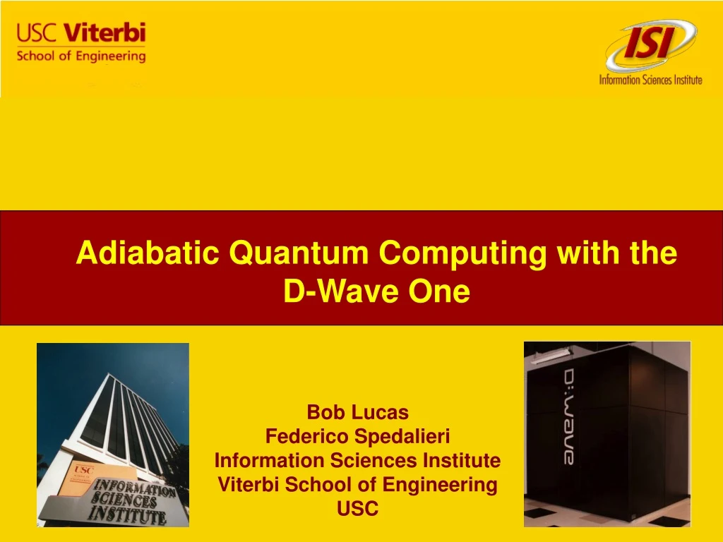
1. Adiabatic Quantum Computing with the D-Wave One Bob Lucas Federico Spedalieri Information Sciences Institute Viterbi School of Engineering USC 1

2. The End of Dennard Scaling

3. Need More Capability? Massive Scaling – ORNL Cray XK7 Exploit a New Phenomenon Adiabatic Quantum Processor D-Wave One Application Specific Systems D.E. Shaw Research Anton

4. Overview • Adiabatic quantum computation • Brief description of D-Wave One • The three main thrusts of research: Quantumness Benchmarking Applications

5. E gmin E1 E0  0 1 Adiabatic Quantum Computation . . . Quantum computer Hamiltonian: H(t) = (1-(t))H0 + (t)H1 • Prepare the computer in the ground state ofH0 • Slowly vary (t) from 0 to 1 • Read out the final state: the ground state ofH1 • Runtime associated with (gmin)-2 . . .

6. Adiabatic Quantum Optimization • Adiabatic QC is universal (can compute any function, just like circuit model) • But universalitymay be too much to ask for. • Consider only “classical” final Hamiltonians, i.e.: Diagonal (in computational basis) Off-diagonal (in computational basis) The final state is a classical state that minimizes the energy of H1

7. Solving Ising models with AQC • Ising problem: Find • Adiabatic quantum optimization:

8. Overview • Adiabatic quantum computation • Brief description of D-Wave One • The three main thrusts of research: Quantumness Benchmarking Applications

9. USC/ISI’s D-Wave One128 (well, 108) qubit Rainier chip 20mK operating temperature 1 nanoTesla in 3D across processor

10. Qubitsand Unit Cell One qubit SC loop; qubit = flux generated by Josephson current Unit cell compound-compound Josephson junction (CCJJ) rfSQUIDs  flux qubit

11. Eight Qubit Unit Cell

12. Tiling of Eight-Qubit Unit Cells

13. Adiabatic Quantum Optimization Problem: find the ground state of Use adiabatic interpolation from transverse field (Farhi et al., 2000) Graph Embedding implemented on DW-1 via Chimera graph retains NP-hardness V. Choi (2010)

14. Program API

15. Overview • Adiabatic quantum computation • Brief description of D-Wave One • The three main thrusts of research: Quantumness Benchmarking Applications

16. Experimental Quantum Signature (S. Boixo, T. Albash, F. S., N. Chancellor, D. Lidar) 16

17. Classical Simulated Annealing Minimizing a complex cost function we can get trapped in local minima. Add temperature to go “uphill”. Temperature decreases with time.

18. Quantum resources: tunneling

19. Degenerate Ising Hamiltonian +/- 1 -1 +1 -1 -1 1 -1 1 -1 -1 +/- 1 -1 -1 +/- 1 1 -1 1 17-fold degenerate ground space: +/- 1 -1

20. Classical Thermalization 20

21. Several SA schedules

22. Quantum annealing 22

23. Quantum Annealing We want to find the ground state of an Ising Hamiltonian: Instead of “temperature” fluctuations, we use quantum fluctuations a transverse field Slowly remove the transverse field to stay on the ground state:

24. DW1 Gap Gap 1.5 GHz (Temp: 0.35 GHz) Transitions to 4th order in Small gap -> small coupling!!!

25. QA closed system

26. QA open system

27. QA vs. SA

28. Experiments 28

29. Embedding Chip Connectivity Our Quantum Signature problem as it looks in the chip

30. DW1 Experiments 144 embeddings Quantum Signature: this state is suppressed

31. Entanglement 31

32. Entanglement: a definition • Separable states • Entangled states • It is a classical mixture of product states • It can be constructed locally

33. Entanglement in DW2 • Even numerically, determining if a state is entangled is NP-hard • How can we experimentally show entanglement? Measure the complete density matrix of the system Quantum State Tomography Measure an observable that distinguishes entangled states Entanglement Witnesses Separable States • Requires a large number of measurements (exponential in the number of qubits) • The reconstructed density matrix may not be physical (not PSD) • For DW2, these measurements are not even possible • For every entangled state there is an entanglement witness • Measuring the expectation of Z can prove entanglement • But to find Z we need to know the state (or be very lucky) • The measurements required will likely not be available in DW2

34. Magnetic susceptibilities in DW2 • Use a weakly coupled probe to measure • Compute the magnetic susceptibilities as • Use perturbation theory (and some assumptions) to write

35. Separability criteria • Apply PPTSE separability criteria to this general state • All separable states have a PPTSE for any k • Search for PPTSE can be cast as a semidefinite program • Produces a hierarchy of separability tests • If state is entangled, dual SDP computes an entanglement witness

36. Separability criteria with partial information • Some properties of this approach: If the test fails the state may still be entangled We can use a dual approach that checks if a state satisfying the linear constraints is separable (also a SDP) If both tests fail, we need to go to higher k All entangled states will be detected for some k Going beyond k=2 may be tricky (the size of the SDP gets too big) In theory, this is the best you can do with partial information: if you could run the tests for all k, this approach will eventually prove that all states satisfying the linear constraints are entangled or that there is one such state that is separable

37. Overview • Adiabatic quantum computation • Brief description of D-Wave One • The three main thrusts of research: Quantumness Benchmarking Applications

38. Benchmarking 38

39. Benchmarking hard problems10 – 108 qubits

40. Benchmarking hard problems108 qubits, 5us – 20ms

41. Classical repetition cost r

42. Some benchmarking Exponential run time for the best exact classical solver Faster exponential run time for the D-Wave (Vesuvius)

43. Some benchmarking (3BOP h and J)

44. Overview • Adiabatic quantum computation • Brief description of D-Wave One • The three main thrusts of research: Quantumness Benchmarking Applications

45. Some NP-complete problems and their applications The problem addressed by quantum annealing is NP-Complete

46. Given a: Finite transition system M A temporal property p The model checking problem: Does Msatisfy p? It typically requires analyzing every possible path the system can take Workarounds: Binary Decision Diagrams (BDDs) Abstractions The Model Checking Problem Complexity is exponential on the number of states State space explosion problem

47. Abstraction Group states together Eg., localization: neglect some state variables (make them invisible) Eliminate details irrelevant to the property • Obtain smaller models sufficient to verify the property using traditional model checking tools • Disadvantage: • Loss of Precision • False positives/negatives Spurious counterexamples

48. Counterexample-Guided Abstraction-Refinement (CEGAR) Build New Abstract Model Model Check M M’ Pass No Bug Fail Check Counterexample Obtain Refinement Cue Real CE Spurious CE Bug ILP Machine learning SAT AQC

49. Summary • DW1 is a programmable superconducting quantum adiabatic processor • It solves a particular type of combinatorial optimization problem • We have investigated the quantum nature of the device • We chose a problem for which classical thermalization and quantum annealing predict different statistics • Experiments agree with quantum annealing prediction suggesting quantum annealing is surprisingly robust against noise • Working on an experimental test for entanglement • Benchmarks show promising scaling when compared with classical solvers • Currently working to bridge the gap between the device and real applications (non-trivial issues to be addressed)