Download
1 / 17
170 likes | 193 Views
Detailed study on hydraulic impedance testing in water disposal wells in Oman, including wellbore diagrams, surface pressure responses, fracture simulations, pulse reflections, fracture length calculations, fracture geometries, and closure stress measurements.

E N D
Simulated surface pressure response for a single diameter wellbore with no fracture. Notice that surface pressure never rises above its original value.
Simulated surface pressure response of an infinite acting fracture. Notice how the reflection from the fracture changes from positive to negative because of the negative reflection of an open fracture.
Calculated response of SH-F3 wellbore and fracture to HIT pulse.
Well SH3-1 Example of recorded HIT data before processing shows high frequency component caused by hanging pipe and low frequency oscillation caused by initial shut-in water hammer.
Well SH3-1 Example of filtered and de-trended data for the same pulse - has removed the high frequency component, and the sinusoidal oscillation - making the pulse reflections in the signal much clearer.
Plot of pulse from SH3-1 first shut-in showing location of possible tip reflection.
Idealized tip reflection and method for calculating fracture length using tip reflection. Time between reflection from fracture mouth and fracture tip, divided by two, multiplied by wave velocity in the fracture gives estimate of fracture length.
Example pulse from SH3-2 first shut-in, showing reflection from casing/open-hold interface and multiple fracture reflections.
Plot of Reflection Coefficient (ignoring wellbore attenuation) shows how it is insensitive to the controlling fracture dimension (either length or height) once this dimension is greater than about 10 meters. Once that dimension is greater than 10 meters, the hydraulic impedance of the fracture is so small compared to that of the wellbore that the reflection coefficient is almost -1.
Possible fracture geometries leading to multiple reflections of the HIT pressure pulse.
Summary of results on frac dimensions: • Length 11-12 m (tip reflections) • Two identified frac initiation points per well • Upper at ca. 1230 m, lower at ca. 1360 m
Plot of surface pressure versus reflection coefficient for SH3-1 fourth shut-in. Closure is estimated between pulses at 798 and 919 psi.
Plot of surface pressure versus reflection coefficient for SH3-2 third shut-in. Fracture closure estimated to at 1165 to 1220 psi.
Closure stresses as measured by HIT: • Well 1: 858, 898, 901, 859 psi. Av. 0.63 psi/ft • Well 2: 1183, 1255, 1193 psi. Av. 0.74 psi/ft • Closure stresses as measured by pressure fall-off analysis: • Well 1: 880 psi • Well 2: 1210 psi