Download
1 / 16
160 likes | 177 Views
B-Trees are multi-way search trees commonly used in database systems or other applications where data is stored externally on disks and keeping the tree shallow is important.

E N D
B-Trees CSE 373 Data Structures
Readings • Reading Chapter 14 • Section 14.3 • See also (2-4) trees Chapter 10 Section 10.4 B-trees
B-trees • Invented in 1972 by Rudolf Bayer (-) and Ed McCreight(-) B-trees
13:- 17:- 6:11 6 7 8 11 12 3 4 13 14 17 18 Beyond Binary Search Trees: Multi-Way Trees • Example: B-tree of order 3 has 2 or 3 children per node • Search for 8 B-trees
B-Trees B-Trees are multi-way search trees commonly used in database systems or other applications where data is stored externally on disks and keeping the tree shallow is important. A B-Tree of order M has the following properties: 1. The root is either a leaf or has between 2 and M children. 2. All nonleaf nodes (except the root) have between M/2 and M children. 3. All leaves are at the same depth. All data records are stored at the leaves. Internal nodes have “keys” guiding to the leaves. Leaves store between M/2 and M data records. B-trees
ki k1 ki-1 kM-1 . . . . . . B-Tree Details Each (non-leaf) internal node of a B-tree has: • Between M/2 and M children. • up to M-1 keys k1 <k2 < ... <kM-1 Keys are ordered so that: k1 <k2 < ... <kM-1 B-trees
B-tree alternate definitions • There are several definitions • What was in the previous slide is the original def. • The textbook has a slightly different one B-trees
k 1 Properties of B-Trees Children of each internal node are "between" the items in that node. Suppose subtree Ti is the ith child of the node: all keys in Ti must be between keys ki-1 and ki i.e. ki-1£ Ti < ki ki-1 is the smallest key in Ti All keys in first subtree T1 < k1 All keys in last subtree TM ³ kM-1 k k . . . k k k k . . . M-1 i-1 i i . . . . . . T T T T T T 1 1 i i M B-trees
Example: Searching in B-trees • B-tree of order 3: also known as 2-3 tree (2 to 3 children) • Examples: Search for 9, 14, 12 • Note: If leaf nodes are connected as a Linked List, B-tree is called a B+ tree – Allows sorted list to be accessed easily 13:- - means empty slot 17:- 6:11 6 7 8 11 12 3 4 13 14 17 18 B-trees
13:- 17:- 6:11 6 7 8 11 12 3 4 13 14 17 18 Inserting into B-Trees • Insert X: Do a Find on X and find appropriate leaf node • If leaf node is not full, fill in empty slot with X • E.g. Insert 5 • If leaf node is full, split leaf node and adjust parents up to root node • E.g. Insert 9 B-trees
After insert of 5 and 9 11 13 6 - 11 - 17 - 6 7 8 9 11 12 13 14 17 18 3 4 5 B-trees
13:- 17:- 6:11 6 7 8 11 12 3 4 13 14 17 18 Deleting From B-Trees • Delete X : Do a find and remove from leaf • Leaf underflows – borrow from a neighbor • E.g. 11 • Leaf underflows and can’t borrow – merge nodes, delete parent • E.g. 17 B-trees
13:- 17:- 6:8 6 7 8 12 3 4 13 14 17 18 Deleting case 1 “8” was borrowed from neighbor. Note the change in the parent B-trees
Deleting Case 2 8 - 6 - 13 - 8 12 13 14 18 3 4 6 7 B-trees
Run Time Analysis of B-Tree Operations • For a B-Tree of order M • Each internal node has up to M-1 keys to search • Each internal node has between M/2 and M children • Depth of B-Tree storing N items is O(log M/2 N) • Find: Run time is: • O(log M) to binary search which branch to take at each node. But M is small compared to N. • Total time to find an item is O(depth*log M) = O(log N) B-trees
Summary of Search Trees • Problem with Binary Search Trees: Must keep tree balanced to allow fast access to stored items • AVL trees: Insert/Delete operations keep tree balanced • Splay trees: Repeated Find operations produce balanced trees • Multi-way search trees (e.g. B-Trees): More than two children • per node allows shallow trees; all leaves are at the same depth • keeping tree balanced at all times B-trees