Exploring Newton-Cotes Formulas for Numerical Integration
Learn about Newton-Cotes formulas for numerical integration, including Trapezoid, Simpson's, and Midpoint rules, with examples and MATLAB programs. Discover Gaussian quadrature and references for further study.

Exploring Newton-Cotes Formulas for Numerical Integration
E N D
Presentation Transcript
Numerical Integration Dr. Asaf Varol
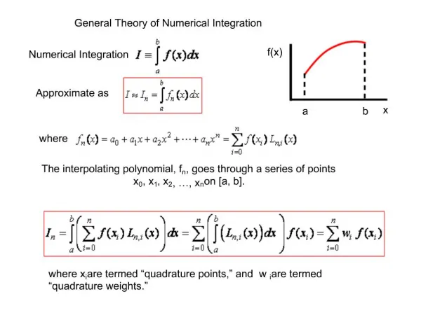
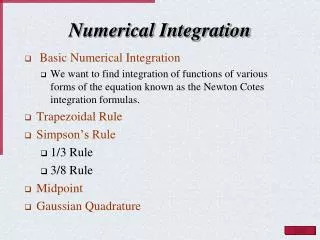
Numerical Integration • Numerical integration is a primary tool used for definite integrals that cannot be solved analytically. A numerical integration rule has the form • we investigate several basic quadrature formulas that use function values at equally spaced points; these methods are known as Newton-Cotes formulas. There are two types of Newton –Cotes formulas, depending on whether or not the function values at the ends of the interval of integration are used. The trapezoid and Simpson rules are examples of “closed” formulas, in which the endpoint values are used. The midpoint rule is the simplest example of an “open” formula, in which the endpoints are not used [2].
Newton-Cotes Closed FormulasTrapezoid Rule • One of the simplest ways to approximate the area under a curve is to approximate the curve by a straight line. The trapezoid rule approximates the curve by the straight line that passes through the points [a, f(a) and b, f(b)], the two ends of the interval of interest. We have x0=a, x1=b, and h=b-a, and then
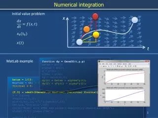
Figure • Figure given on the right side compares the actual value of the area with that found by using the midpoint rule. The area given by the integral S (hatched) and the approximation using the midpoint rule (shaded) [2].
References • Celik, Ismail, B., “Introductory Numerical Methods for Engineering Applications”, Ararat Books & Publishing, LCC., Morgantown, 2001 • Fausett, Laurene, V. “Numerical Methods, Algorithms and Applications”, Prentice Hall, 2003 by Pearson Education, Inc., Upper Saddle River, NJ 07458 • Rao, Singiresu, S., “Applied Numerical Methods for Engineers and Scientists, 2002 Prentice Hall, Upper Saddle River, NJ 07458 • Mathews, John, H.; Fink, Kurtis, D., “Numerical Methods Using MATLAB” Fourth Edition, 2004 Prentice Hall, Upper Saddle River, NJ 07458 • Varol, A., “Sayisal Analiz (Numerical Analysis), in Turkish, Course notes, Firat University, 2001