Download
1 / 50
560 likes | 938 Views
Learn to import raw RNA-seq data into Galaxy, perform quality control, trim reads, map to genome, and analyze differential gene expression to understand impact of plant parasitic nematodes. Explore key nematodes causing agricultural damage worldwide. Experiment on plants to study response to nematode infection. Access RNA-seq data at NCBI for analysis.

E N D
RNA-seq data analysis using Galaxy: • Lab 1 Import raw sequence data into Galaxy Quality control and trimming of RNAseq reads Mapping reads to the genome Differential gene expression analysis; biological meaning
Plant Parasitic Nematodes • >4000 species of plant parasitic nematodes • Collectively, these nematodes cause >$80 billion in damage to agricultural crops worldwide every year • Most live in soil and damage plant roots Burrowing nematodes in red clover roots Tree die-off caused by pine wilt nematode Root knot nematode damage in tomato
The Beet Cyst Nematode • Insert image of beet cyst nematode life cycle here, example can be found at • http://soybeanresearchinfo.com/diseases/scn.html • (see “Life Cycle dropdown menu) https://www.youtube.com/watch?v=VxrwutAew2I • Insert image of beet cyst nematode crop damage here, example can be found at https://www.forestryimages.org/browse/subthumb.cfm?sub=13001&Arc=5
Experimental question • How do plants respond to beet cyst nematode infection? http://apsjournals.apsnet.org/doi/full/10.1094/MPMI-07-15-0156-R
Experimental design • Treatment: plants infected with nematodes vs. uninfected plants • Time of exposure: 4 days post-infection vs. 10 days post-infection • Plant genotype: wild-type vs. arr3,4,5,6,7,8,9,15 (mutant plant that cannot produce cytokinin hormones) zeatin
Experimental design 4 d.p.i./10 d.p.i Infected/Uninfected Wild-type/arr3,4,5,6,7,8,9,15 • All combinations of the three variables were examined • Which variable is most critical to answering our experimental question? • Which variables should be held constant?
Our experimental data set Wild-type plants 4 days WT-INF1 WT-INF2 WT-INF3 WT-CON1 WT-CON2 WT-CON3 • Isolated RNA from roots • Performed RNA-seq using an Illumina HiSeq2500 • 50 nt single-end reads
Accessing RNA-seq data at NCBI Shanks et al. (2016) deposited sequence data from their study at NCBI. What NCBI Bioproject number is associated with this work?
Accessing RNA-seq data at NCBI NCBI Sequence Read Archive (SRA): Repository for “raw” next generation sequencing data
Descriptors: • Col (wild type) vs. Type-A (arr3,4,5,6,7,8,9,15) • Infected vs. non-infected • 4 dpi vs. 10 dpi • Rep (Biological Replicate 1, 2, or 3) Select Wild type, infected, 4 dpi, Biological replicate 3
Downloading sequence data • Very large files! • File above contains 11.1 million sequence reads, and each sequence read is 50 nt long • ~2 Gb file size: Transfer, storage, and analysis of a file this large is a major issue! • FASTA format vs FASTQ format
FASTA format >ID line(s) SEQUENCE
FASTQ format @ID line SEQUENCE +Secondary ID (optional) Quality Score for base directly above (in ASCII format) Base = T Quality score = “:” = 25 • Quality score represents confidence that a particular base is called correctly: • Quality score X = error probability of 10-X/10
FASTQ format Calculating a base quality score from an ASCII symbol Base = G Quality score = “?” “?” = 63 (see ASCII table) ASCII value – 33 = Quality score 63 – 33 = 30 Quality score of 30 is an expected error rate of 10-3
Easily transferring, storing, and analyzing next-gen sequencing data: Galaxy Tool menu Interface for selected tool History
Galaxy Main (web interface) provides: • Access to hundreds of advanced, open source sequence analysis tools, all with a GUI (no programming expertise needed) • Data storage (200 Gb per registered user) • Simple pathways to import data from NCBI or personal computer • Substantial “back end” computing power to run analyses (Texas Advanced Computing Center) • Tech support from staff and “Galaxy community” (Galaxy Biostars) • Stable, but updated infrastructure (12 years old, supported by NSF and NIH)
Introduction to Galaxy- Lab 1 • RNAseq tutorial Part 1: • Get a Galaxy user account • Galaxy User Interface (UI) “tour” • Import WT-CON1 or WT-INF1 SRR files from NCBI • Import Arabidopsis genome annotation file (TAIR10 GTF)
RNA-seq data analysis using Galaxy • Part 2 Import raw sequence data into Galaxy Quality control and trimming of RNAseq reads Mapping reads to the genome Differential gene expression analysis; biological meaning
Assessing the quality of Illumina sequence data- FastQC • FastQC • Basic stats: # reads, sequence lengths • Base quality scores across all reads • Adapter sequence contamination
High quality sequence run Average quality scores at each position in the sequence read
Not relevant for RNA seq data, where reads will be highly repetitive/redundant (e.g. high abundance transcripts)
Removing/trimming low quality reads- Trimmomatic • Trimmomatic • Removes any sequences derived from the Illumina adapters • Performs sliding window trimming: removes blocks of low quality sequence from the ends of the reads (e.g. 4 nt window with average quality score < 20) • Minimum length trimming: after completion of steps 1 and 2, removes any sequences shorter than a specified length (e.g. 25 nt) • Insert conceptual image of quality trimming here, example can be found at https://www.slideshare.net/afgane/introduction-to-galaxy-and-rnaseq • (slide 67)
Mapping the reads to the reference genome- HISAT2 • We need to match our RNA-seq reads back to the genome (What gene was this RNA molecule transcribed from?) • Pairwise alignment problem • BLASTN? Too slow • HISAT2- specifically designed to rapidly align RNA-seq reads to a genome sequence • Insert conceptual image of read alignment here, example can be found at https://www.hindawi.com/journals/bmri/2010/853916/fig5/
Mapping the reads to the reference genome- HISAT2 • HISAT2 output: Mapping Summary Did not align to genome Aligned at more than one location in the genome (multi-mappers) % of reads that aligned to at least one location in the genome
Mapping the reads to the reference genome- HISAT2 • HISAT2 output: a BAM file (Binary Alignment/Mapping) Matching chromosome Sequence name Position on chromosome (first base) • “Flag codes” • 0 = matches forward strand • 16 = matches reverse strand • 4 = does not match (unmapped)
Visualization of a BAM • mapping file on a • genome browser
Making a counts table- FeatureCounts • FeatureCounts takes each mapped read and assigns it to a specific gene • Uses the match coordinates in the BAM file and the precise gene exon coordinates defined by the Arabidopsis genome annotation (GTF) file
Automating the computational workflow Galaxy allows the creation of computational pipelines (workflows), where the output of one computational analysis is automatically used as an input into the next computational step
RNA-seq data analysis using Galaxy • Part 3 Import raw sequence data into Galaxy Quality control and trimming of RNAseq reads Mapping reads to the genome Differential gene expression analysis; biological meaning
Differential gene expression analysis- DESeq2 • Counts tables = raw input for analysis of differential gene expression • Key question: Which of these genes show a statistically significant difference in counts (transcript abundance) between the experimental samples and the control samples? • Approach: DESeq2- A statistical analysis • package specifically designed for • RNA-seq data
DESeq2- key steps • Normalization • There can be substantial variation in the number of reads mapped in different samples • Thus, raw counts data needs to be normalized to prevent systemic bias in “high count” or “low count” samples
Median centering normalization Counts in sample “X” are multiplied by: Median number of mapped counts across all samples Number of mapped counts in sample “X” 1662 991 947 925 905 848 Median of total mapped counts: 936 Normalized counts for At1G01010 45.53 39.98 36.42 101.06 94.11 114.65
DESeq normalization Step 1: Individually for each gene, calculate the ratio of sample read count to the average read count Sample counts/average counts
DESeq normalization Step 2: For each sample, determine the median of the ratios (a.k.a. scaling factor) and divide this number by all counts values Normalized counts for At1G01010 52.32 44.10 39.75 113.82 108.33 133.33
DESeq2- key steps • 2. Hypothesis testing • Is the distribution of counts in the • control samples significantly different • than the distribution of counts in the • infected samples? • Initial P-value calculation based on • Wald test
DESeq2- key steps • Correction for multiple hypothesis testing (false positive problem) • In DESeq2, this involves adjusting the P-values for each comparison to limit false discovery rate • Bonferroni correction: P * number of hypothesis tests • Benjamini-Hochberg correction: P * P-value corrected with Benjamini-Hochberg Average counts across all samples Fold change (Log2) Standard error Wald statistic Gene name P-value Number of hypothesis tests DESeq2 results file P-value ranking
DESeq- key steps • Calculate fold-change in gene expression: • Fold change = Total counts experimental/total counts control • Fold change is often Log2 transformed
DESeq- key steps • Visualization tools/tests • MA plot- Counts (expression level) vs. fold-change; colored dots are statistically significant differences • PCA plots- Method to visualize overall data similarity between samples; groupings based on treatment are expected
Defining differential gene expression • Defining a differentially expressed gene • P-value: Typically adjusted P-value ≤ 0.05 or ≤ 0.01 • Fold change: Typically a minimum fold-change is considered (e.g. 2-fold)
I have “the list”- now what? • Need to define the overall functions of the differentially expressed genes- what is the biological meaning of these changes? • Need annotations for the gene list • What Biological Processes, Molecular Functions, and Cellular Components (GO Categories) are (over)represented in my gene list? Panther provides functions/GO term information for any gene list
Panther and GO category enrichment • GO category over-representation analysis tells us which biological processes are particularly affected by our experimental treatment • Analysis of a list of 80 differentially expressed genes Expected number of genes in this category, if we randomly selected 80 genes from the entire Arabidopsis genome (27,352 genes) Number of genes in the entire Arabidopsis genome that are classified in this GO category Associated P value GO Biological Process Category Number of genes in the provided gene list (80 differentially expressed genes) that are classified in this GO category Fold enrichment (+) or depletion (-) of this GO category in the gene list, compared to random chance
Now the real work begins… • Results of transcriptome studies help us to generate new (non-obvious) hypotheses regarding gene function, gene regulation, etc. • These hypotheses need to be developed and supported with a thorough review of the primary literature in the field, and potentially new targeted experiments. • Gene expression profiling allows us to make novel connections between seemingly unrelated biological processes