Download
1 / 32
320 likes | 391 Views
Explore the concepts, facts, and applications of Probabilistic Turing Machines and Probabilistic Algorithms. Understand BPP, error probabilities, and Randomized Polynomial Time complexity. Discover why probabilistic algorithms are valuable and how they are used in various scenarios.

E N D
Probabilistic Turing Machines Stephany Coffman-Wolph Wednesday, March 28, 2007
Probabilistic Turing Machine • There are several popular definitions: • A nondeterministic Turing Machine (TM) which randomly chooses between available transitions at each point according to some probability distribution • A type of nondeterministic TM where each nondeterministic step is called a coin-flip step and has two legal next moves • A Turing Machine in which some transitions are random choices among finitely many alternatives • Also known as a Randomized Turing Machine
TM Specifics • There are (at least) three tapes • 1st Tape holds the input • 2nd Tape (also known as the random tape) is covered randomly (and independently) with 0’s and 1’s • ½ probability of a 0 • ½ probability of a 1 • 3rd Tape is used as the scratch tape
When a Probabilistic TM Recognizes a Language • Accept all strings in the language • Reject all strings not in the language • However, a probabilistic TM will have a probability of error
Probabilistic TM Facts • Each “branch” in the TMs computation has a probability • Can have stochastic results • Hence, on a given input it: • May have different run times • May not halt • Therefore, it may accept the input in a given execution, but reject in another execution • Time and space complexity can be measured using the worst case computation branch
Probabilistic Algorithm • Also known as Randomized Algorithms • An algorithm designed to use the outcome of a random process • In other words, part of the logic for the algorithm uses randomness • Often the algorithm has access to a pseudo-random number generator • The algorithm uses random bits to help make choices (in hope of getting better performance)
Why use Probabilistic Algorithms? • Probabilistic algorithms are useful because • It is time consuming to calculate the “best” answer • Estimation could introduce an unwanted bias that invalidates the results • For example: Random Sampling • Random sampling is used to obtain information about individuals in a large population • Asking everyone would take too long • Querying a not random selected subset might influence (or bias) the results
BPP • Bounded error Probability in Polynomial time • Definition: • The class of languages that are recognized by probabilistic polynomial time TM with an error probability of 1/3 (or less) • Or another way say it: • The class of languages that a probabilistic TM halts in polynomial time with either a accept or reject answer at least 2/3 of the time
A Problem in BPP: • Can be solved by an algorithm that is allowed to make random decisions (called coin-flips) • Guaranteed to run in polynomial time • On a given run of the algorithm, it has a (at most) 1/3 probability of giving an incorrect answer • These algorithms are known as probabilistic algorithms
Why 1/3? • Actually, this is arbitrary • In fact can be any constant between 0 and ½ (as long as it is independent of the input) • Why? • If the algorithm is run many times, the probability of the probabilistic TM being wrong the majority of the time decreases exponentially • Therefore, these kinds of algorithms can become more accurate by running it several times (and then taking the majority vote of the results)
To Illustrate the Concept • Let the error probability be 1/3 • We have a box containing many red and blue balls • 2/3 of the balls are one color • 1/3 of the balls are the other color • (But, we don’t know which color is 2/3 or which color is 1/3) • To find out, we start taking samples at random and keep track of which color ball we pulled from the box • The color that comes up most frequently during a large sampling will most likely be the majority color originally in the box
How This Relates… • The blue and red balls correspond to branches in a probabilistic (polynomial time) TM. Lets call it M1 • We can assign each color: • Red = accepting • Blue = rejecting • The sampling can be done by running M1 using another probabilistic TM (lets call it M2) with a better error probability • M2’s error probability is exponentially small if it runs M1 a polynomial number of times and outputs the result that occurs most often
Formally: • Let the error probability (Є) be a fixed constant strictly between 0 and ½ • Let poly(n) be any polynomial • For any poly(n), a probabilistic polynomial time TM M1 that operates with error probability Є has an equivalent probabilistic polynomial time TM M2 • This TM M2 has an error probability of 2-poly(n)
RP • Randomized Polynomial time • A class of problems that will run in polynomial time on a probabilistic TM with the following properties: If the correct answer is • no, always return no • yes, return yes with probability at least ½ • Otherwise, returns no • Formally • The class of languages for which membership can be determined in polynomial time by a probabilistic TM with no false acceptances and less than half of the rejections are false rejections
Facts About RP • If the algorithm returns a yes answer, then yes is the correct answer • If the algorithm returns a no answer, then it may or may not be correct • The ½ in the definition is arbitrary • Like we saw in the BPP class, running the algorithm addition repetitions will decrease the chance of the algorithm giving the wrong answer • Often referred to as a Monte-Carlo Algorithm (or Monte-Carlo Turing Machine)
Monte Carlo Algorithm • A numerical Monte Carlo method used to find solutions to problems that cannot easily to solved using standard numerical methods • Often relies on random (or pseudo-random) numbers • Is stochastic or nondeterministic in some manner
Co-RP • A class of problems that will run in polynomial time on a probabilistic TM with the following properties: If the correct answer is • yes, always return yes • no, return no with probability at least ½ • Otherwise, returns a yes • In other words: • If the algorithm returns a no answer, then no is the correct answer • If the algorithm returns a yes answer, then it may or may not be correct
ZPP • Zero-error Probabilistic Polynomial • The class of languages for which a probabilistic TM halts in polynomial time with no false acceptances or rejections, but sometimes gives an “I don’t know” answer • In other words: • It always returns a guaranteed correct yes or no answer • It might return an “I don’t know” answer
Facts About ZPP • The running time is unbounded • But it is polynomial on average (for any input) • It is expected to halt in polynomial time • Similar to definition of P except: • ZPP allows the TM to have “randomness” • The expected running time is measured (instead of the worst-case) • Often referred to as a Las-Vegas algorithm (or Las-Vegas Turning Machine)
Las Vegas Algorithm • A randomized algorithm that never gives an incorrect result. It either produces a result or fails • Therefore, it is said that the algorithm “does not gamble” with it’s result. It only “gambles” with the resources used for computation
L, ¬ L, and ZPP • If L is in ZPP, then ¬ L is in ZPP • Where ¬ L represents the complement of L • Why? • If L is accepted by TM M that is in ZPP. • We can alter M to accept ¬ L by • Turning the acceptance by M into halting without acceptance • If M halted without accepting before, instead we accept and halt
Relationship Between RP and ZPP • ZPP = RP co-RP • Proof Part 1: RP co-RP is in ZPP • Let L be a language recognized by RP algorithm A and co-RP algorithm B • Let w be in L • Run w on A. If A returns yes, the answer must be yes. If A returns no, run w on B. If B returns no, then the answer must be no. Otherwise, repeat. • Only one of the algorithms can ever give a wrong answer. The chance of an algorithm giving the wrong answer is 50%. • The chance of having the kth repetition shrinks exponentially. Therefore, the expected running time is polynomial • Hence, RP intersect co-RP is contained in ZPP
Relationship Between RP and ZPP • ZPP = RP co-RP • Proof Part 2: ZPP is contained in RP co-RP • Let C be an algorithm in ZPP • Construct the RP algorithm using C: • Run C for (at least) double its expected running time. • If it gives an answer, that must be the answer • If it doesn’t given an answer before the algorithm stops, then the answer is no • The chance that algorithm C produces an answer before it is stopped is ½ (and hence fitting the definition of an RP algorithm) • The co-RP algorithm is almost identical, but it gives a yes answer if C does produce an answer. • Therefore, we can conclude that ZPP is contained in RP co-RP
What We Can Also Conclude • As seen in the proof of ZPP = RP co-RP we can conclude that • ZPP RP • ZPP co-RP
Relationship Between P and ZPP • P ZPP • Proof • Any deterministic, polynomial time bounded TM is also a probabilistic TM that ignores its special feature that allows it to make random choices
Relationship Between NP and RP • RP NP • Proof • Let M1 be a probabilistic TM in RP for language L • Construct a nondeterministic TM M2 for L • Both of these TMs are bounded by the same polynomial • When M1 examines a random bit for the first time, M2 chooses both possible values for the bit and writes it on a tape • M2 will accept whenever M1 accepts. M2 will not accept otherwise
Relationship Between NP and RP • Proof continued • Let w be in L • M1 has a 50% probability of accepting w. • There must be some sequence of bits on the random tape that leads to the acceptance of w • M2 will choose that sequence of bits and accepts when the choice is made. Thus, w is in the language of M2 • If w is not in L, then there is no sequence of random bits that will make M1 accept. Therefore, M2 cannot choose a sequence of bits that leads to acceptance. Thus, w is not in the language of M2
Where Does BPP Fit in? • It is still an open question whether NP is a subset of BPP or BPP is a subset of NP • However, it is believed that RP is a subset of BPP
Why Study Probabilistic TM? • To attempt to answer the question: • Does randomness add power? • Or putting it another way: • Are there problems that can be solved by a probabilistic TM (in polynomial time) but these same problems cannot be solved by a deterministic TM in polynomial time?
Resources • Introduction of the Theory of Computation by Michael Sipser, PWS Publishing Company, 1997 • Introduction to Automata Theory, Languages, and Computation by Hopcroft, Motwani, and Ullman, Person Education, Inc, 2006 • Introduction to the Theory of Computation by EitanGurari, Computer Science Press, 1989 (http://www.cse.ohio-state.edu/~gurari/theory-bk/theory-bk.html) • “Dictionary of Algorithms and Data Structures”, NIST website (http://www.nist.gove/dads/) • “Probabilistic Turing Machines”, “Randomized algorithm”, “BPP”, “ZPP”, “CP”, “Monte Carlo algorithm”, and “Las Vegas algorithm”, Wikipedia website (http://en.wikipedia.org/)